<- previous index next ->
Some partial differential equations are difficult to solve symbolically
and some are difficult to solve numerically.
This lecture covers the numerical solution of simple partial
differential equations where the initial conditions values are known.
See simple definitions .
We know from lectures on derivatives:
Given a function U(x,y) and points x0, x1, x2, y0, x1=x0+h, x2=x1+h
dU(x0,y0)/dx = Ux(x0,y0) = (-3*U(x0,y0) +4*U(x1,y0) -1*U(x2,y0) )/ 2h
Ux(x1,y0) = (-1*U(x0,y0) +1*U(x2,y0) )/ 2h
Ux(x2,y0) = ( 1*U(x0,y0) -4*U(x1,y0) +3*U(x2,y0) )/ 2h
adding ------------------------------------------------------
Ux(x0,y0)+U(x1,y0)+Ux(x2,y0) = (-3*U(x0,y0) +3*U(x2,y0)) /2h
divide by 3
rearrange U(x2,y0) = U(x0,y0) + 2*h*(Ux(x0,y0)+U(x1,y0)+Ux(x2,y0))/3
Thus we have a way to compute a new value of U, knowing a previous value
and derivatives. Changing the notation to go from point xa to xb=xa+hx :
U(xb,y0) = U(xa,y0) + hx*(Ux(xa,y0)+Ux(xa+hx/2,y0)+Ux(xa+hx,y0))/3
Sample test case for above
source code pde_i1.java
source code pde_i1_java.out
We are told there is an unknown function U(x,y) that satisfies
the a differential equation:
Given the value of U(x0,y0) only one point
Given a computable function Ux(x,y)
Given a computable function Uy(x,y)
We can compute U(x,y) at an array of points x0 to xmax, y0 to ymax
with step size hx and hy.
Sample test case for above
source code pde_i2.java
source code pde_i2_java.out
PDE with computable Ux(x,y) and U(y(x,y) and known U(x0,y0)
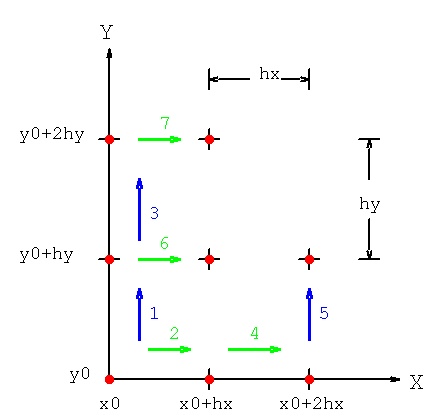 1 compute U(x0,y0+hy) = U(x0,y0) + hy*Uy(x0,y0) or higher order method
2 compute U(x0+hx,y0) = U(x0,y0) + hx*Ux(x0,y0)
3 compute U(x0,y0+2*hy) = U(x0,y0+hy) + hy*Uy(x0,y0+hy)
4 compute U(x0+2*hx,y0) = U(x0+hx,y0) + hx*Ux(x0+hx,y0)
5 compute U(x0+2*hx,y0+hy) = U(x0+2*hx,y0) + hy*Uy(x0+2*hx,y0)
6 compute U(x0+hx,y0+hy) = U(x0,y0+hy) + hx*Ux(x0,y0+hy)
7 compute U(x0+hx,y0+2*hy) = U(x0,y0+2*hy) + hx*Ux(x0,y0+2*hy)
A higher order method can use hx/2 and Ux(x0+hx/2,y0+hy/2) etc.
There are two ways to compute U(x0+hy,y0+hy) and many options beyond that.
1 compute U(x0,y0+hy) = U(x0,y0) + hy*Uy(x0,y0) or higher order method
2 compute U(x0+hx,y0) = U(x0,y0) + hx*Ux(x0,y0)
3 compute U(x0,y0+2*hy) = U(x0,y0+hy) + hy*Uy(x0,y0+hy)
4 compute U(x0+2*hx,y0) = U(x0+hx,y0) + hx*Ux(x0+hx,y0)
5 compute U(x0+2*hx,y0+hy) = U(x0+2*hx,y0) + hy*Uy(x0+2*hx,y0)
6 compute U(x0+hx,y0+hy) = U(x0,y0+hy) + hx*Ux(x0,y0+hy)
7 compute U(x0+hx,y0+2*hy) = U(x0,y0+2*hy) + hx*Ux(x0,y0+2*hy)
A higher order method can use hx/2 and Ux(x0+hx/2,y0+hy/2) etc.
There are two ways to compute U(x0+hy,y0+hy) and many options beyond that.
more examples using MATLAB built in ODE solvers
stiff.m MATLAB source code
% stiff.m using ode15s
function stiff()
[t,y]=ode15s(@vdp1000, [0 3000], [2 0]);
plot(t,y(:,1),'-o')
function dydt = vdp1000(t, y)
dydt = [y(2); 1000*(1-y(1)^2)*y(2)-y(1)];
end % vdp1000
end % stiff
 stiff1.m MATLAB source code
% stiff1.m using ode23
% y1' = y2 y2' = (1-y1^2)*y2-y1
function stiff1()
[t,y]=ode23(@vdp, [0 20], [2; 0]);
plot(t,y(:,1),'-o',t,y(:,2),'-o')
title('Solution of van der Pol Equation (\mu = 1) with ODE23');
xlabel('Time t');
ylabel('Solution y');
legend('y_1','y_2')
function dydt = vdp(t, y)
dydt = [y(2); (1-y(1)^2)*y(2)-y(1)];
end % vdp
end % stiff1
stiff1.m MATLAB source code
% stiff1.m using ode23
% y1' = y2 y2' = (1-y1^2)*y2-y1
function stiff1()
[t,y]=ode23(@vdp, [0 20], [2; 0]);
plot(t,y(:,1),'-o',t,y(:,2),'-o')
title('Solution of van der Pol Equation (\mu = 1) with ODE23');
xlabel('Time t');
ylabel('Solution y');
legend('y_1','y_2')
function dydt = vdp(t, y)
dydt = [y(2); (1-y(1)^2)*y(2)-y(1)];
end % vdp
end % stiff1
 ode21.m MATLAB source code
% ode21.m second oder ode with initial conditions
function ode21
% SOLVE d^2x/d^2t + 5*dx/dt - 4 x = sin(10 t)
% initial conditions: x(0) = 0, x'(0)=0
t=0:0.001:3; % time scale
initial_x = 0;
initial_dxdt = 0;
[t,x]=ode45( @rhs, t, [initial_x initial_dxdt] );
plot(t,x(:,1),t,x(:,2));
title('solve d^2x/d^2t + 5*dx/dt - 4 x = sin(10 t)');
xlabel('t');
ylabel('x');
legend('dx_1','dx_2');
function dxdt=rhs(t,x)
dxdt_1 = x(2);
dxdt_2 = -5*x(2) + 4*x(1) + sin(10*t);
dxdt=[dxdt_1; dxdt_2];
end % rhs
end % ode21
ode21.m MATLAB source code
% ode21.m second oder ode with initial conditions
function ode21
% SOLVE d^2x/d^2t + 5*dx/dt - 4 x = sin(10 t)
% initial conditions: x(0) = 0, x'(0)=0
t=0:0.001:3; % time scale
initial_x = 0;
initial_dxdt = 0;
[t,x]=ode45( @rhs, t, [initial_x initial_dxdt] );
plot(t,x(:,1),t,x(:,2));
title('solve d^2x/d^2t + 5*dx/dt - 4 x = sin(10 t)');
xlabel('t');
ylabel('x');
legend('dx_1','dx_2');
function dxdt=rhs(t,x)
dxdt_1 = x(2);
dxdt_2 = -5*x(2) + 4*x(1) + sin(10*t);
dxdt=[dxdt_1; dxdt_2];
end % rhs
end % ode21
 ode_1.m MATLAB source code
% ode_1.m using ode45 with setup
function ode_1
options = odeset('RelTol', 1e-4, 'AbsTol', [1e-4 1e-4 1e-5]);
[T,Y] = ode45(@ridgid, [0 12], [0 1 1], options);
plot(T, Y(:,1), '-', T, Y(:,2), '-.', T, Y(:,3), '.')
title('second order solution with ode45');
xlabel('Time T');
ylabel('Solution Y');
legend('dy_1','dy_2','dy_3');
function dy=ridgid(t, y)
dy = zeros(3, 1); % force a column vector
dy(1) = y(2) * y(3);
dy(2) = -y(1) * y(3);
dy(3) = -0.51 * y(1) * y(2);
end % ridgid
end % ode_1
ode_1.m MATLAB source code
% ode_1.m using ode45 with setup
function ode_1
options = odeset('RelTol', 1e-4, 'AbsTol', [1e-4 1e-4 1e-5]);
[T,Y] = ode45(@ridgid, [0 12], [0 1 1], options);
plot(T, Y(:,1), '-', T, Y(:,2), '-.', T, Y(:,3), '.')
title('second order solution with ode45');
xlabel('Time T');
ylabel('Solution Y');
legend('dy_1','dy_2','dy_3');
function dy=ridgid(t, y)
dy = zeros(3, 1); % force a column vector
dy(1) = y(2) * y(3);
dy(2) = -y(1) * y(3);
dy(3) = -0.51 * y(1) * y(2);
end % ridgid
end % ode_1

<- previous index next ->
-
CMSC 455 home page
-
Syllabus - class dates and subjects, homework dates, reading assignments
-
Homework assignments - the details
-
Projects -
-
Partial Lecture Notes, one per WEB page
-
Partial Lecture Notes, one big page for printing
-
Downloadable samples, source and executables
-
Some brief notes on Matlab
-
Some brief notes on Python
-
Some brief notes on Fortran 95
-
Some brief notes on Ada 95
-
An Ada math library (gnatmath95)
-
Finite difference approximations for derivatives
-
MATLAB examples, some ODE, some PDE
-
parallel threads examples
-
Reference pages on Taylor series, identities,
coordinate systems, differential operators
-
selected news related to numerical computation