[CMSC 455] | [Syllabus] | [Lecture Notes] | [Homework] | [Projects] | [Files] | [Notes, all]
  Homework is submitted when due.
  No late penalty for online course.
 Get any of my files you need on linux.gl.umbc.edu
  cp /afs/umbc.edu/users/s/q/squire/pub/download/some_file.c  .

  Be careful saving a file from a web page. You may have
  to fix broken lines.
 The "submit" facility only works on the "gl" machines.
 The student commands are:
    submit   cs455 hw1 some_file
    submit   cs455 hw1 some_file another_file output_file
    submitrm cs455 hw1 some_file # removes file
    submitls cs455 hw1           # list files

    do not submit  a.out  that is the executable file
    submit  cs455 hw1 txt.out       from  a.out > txt.out  or
    submit  cs455 hw1 hw1.out       from  a.out > hw1.out

    if for some reason just "submit" says no such program, use
    /afs/umbc.edu/common/submit/bin/submit cs455 hw1 some_file
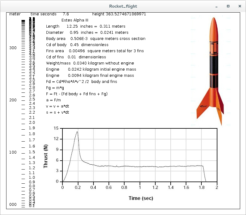
Modeling and simulation: Rocket flight, how high?
In a language of your choice, write the program defined in
lecture 2. Test your program and
produce an output file, then  submit both files
on a GL machine:
(Do not compute at time = 0.0, you will get a negative velocity
  due to force of gravity, first Ft should be 6.0, from array,
  keep computing after time = 1.8 with Ft = 0.0 until V < 0.0 after
  about 7 seconds, about 350 meters, your thrust may be different.)

For each time 0.1, 0.2, ... about 7.0 seconds,
print t time, s altitude, v velocity, a acceleration, F net force, m mass

submit cs455 hw1 your-source your-output

print output as a text file, do not submit  a.out  that is a binary file.
Print every dt=0.1, tenth of a second.
All values are in Metric system. Rho = 1.293

The graphics class sees the flight that produces this as a moving flight
In a language of your choice, write a program that
does a least square fit of the thrust data used in Homework 1.
Use your thrust data  x =  0.0  0.1   0.2  ...  1.8 1.9
                      y =  0.0  6.0  14.1  ...  4.5 0.0
Be sure time 0.0 has value 0.0, time 1.9 has value 0.0

Do the least square fit with 3, 4, ... , 17 degree polynomials.
Compute the maximum error, the average error and RMS error
for each fit. If convenient, look at the plots of your fit
and compare to the input.

Print out your data. Remove excess printout, print:
Print out your polynomial order for each degree 3..17 and
print out maximum, average and RMS error for each.
Lecture 1 shows how to compute error
copy whatever you need from Lecture 4, Least square fit
Note: Python polyfit does not do a least square fit, no "order" parameter.
Many languages covered in Lecture 4, a must read.

If using python, see test_lsfit.py3, lsfit.py3, peval.py3  from download
OK to use my files.

submit your source code file(s) and your output file

submit cs455 hw2 your-source your-output

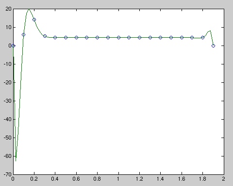
My MatLab errors looked like:hw2_m.out
   (with a lot of complaints from MatLab!)

UGH! Matlab has started blabbing errors. I will ignore them.

Plotting three points between each starting point in MatLab, n=19, gave:


The steps are typically:
Have the thrust data in X array, time values.
Have the thrust data in Y array, newton values.
Build the least square simultaneous equations, n=3 first

Given a value of Y for each value of X,
  Y_approximate =  C0 + C1 * X + C2 * X^2 +  C3 * X^3
Then the linear equations would be:

| SUM(1  *1) SUM(1  *X) SUM(1  *X^2) SUM(1  *X^3) | | C0 |   | SUM(1  *Y) |
| SUM(X  *1) SUM(X  *X) SUM(X  *X^2) SUM(X  *X^3) | | C1 |   | SUM(X  *Y) |
| SUM(X^2*1) SUM(X^2*X) SUM(X^2*X^2) SUM(X^2*X^3) |x| C2 | = | SUM(X^2*Y) |
| SUM(X^3*1) SUM(X^3*X) SUM(X^3*X^2) SUM(X^3*X^3) | | C3 |   | SUM(X^3*Y) |

Note that index [i][j] of the matrix has SUM(X^i*X^j))
for i=0 to 3, j=0 to 3   X^0 = 1   X^1 = X

Solve the simultaneous equations for C0, C1, C2, C3
using some version of "simeq". Remember 4 C values for power 3.
This is equivalent to polyfit.

Compute errors by using "peval" with the coefficients
for each X and subtract the corresponding Y.
Save maximum error, compute average and RMS error.
Print.

Repeat, advancing n to 4, 5, ..., 17

put in time and thrust data from homework 1
k=20          number of data points
x=time[i]
y=thrust[i]
Do some least square polyfit on x,y get C values
use  err_each_term = polyval(pwr, x, C)   all 20
compute max, avg, rms error for each of 20  err_each_term-y[i]

Use lsfit.py3,peval.py3 not polyfit,polyval if you are better with Python 3.
You must understand lecture 4.
See Lecture 9
last name a-j a, last name k-r b,  last name s-z c   ?
cp /afs/umbc.edu/users/s/q/squire/pub/download/q1_455a.doc
cp /afs/umbc.edu/users/s/q/squire/pub/download/q1_455b.doc
cp /afs/umbc.edu/users/s/q/squire/pub/download/q1_455c.doc

answer with libreoffice or Microsoft Word

submit cs455 quiz1 q1_455?.doc  or  q1_455?.docx
1. Compare two methods of integrating  sin(x) from 0 to 1
Take as the exact solution  -cos(1.0)+cos(0.0) = 1.0-cos(1.0)
Print out number of points, your integration computed value, and
your_computed_value - exact_solution the error
Remember lecture 7.

1.a) Use the trapezoidal method with 16, 32, 64 and 128 points.
   Put this in a loop  e.g. in C  for(n=16; n<=128; n=n*2)
   Note how the error decreases as n increases.
   h = 1/n
   your_value = h * ((sin(0)+sin(1.0))/2 + sum i=1..n-1 sin(i*h))

  trapezoide.py sample integration
  trapezoide.java sample integration

1.b) Use the Gauss Legendre method with 8 and 16 points.
   Copy the function  gaulegf  from your choice of language
   or convert to your choice of language. Be sure to keep
   the #undef abs and #define abs in "C" code.

   double x[17], w[17]
   n=8   then again for n=16
   gaulegf(0.0, 1.0, x, w, n)
   your_value = 0.0
   for(j=1; j<=n; j++)
      your_value = your_value + w[j]*sin(x[j])


   Note the significantly smaller error than for trapezoid.

gaulegf.py sample integration
gaulegf.java sample integration


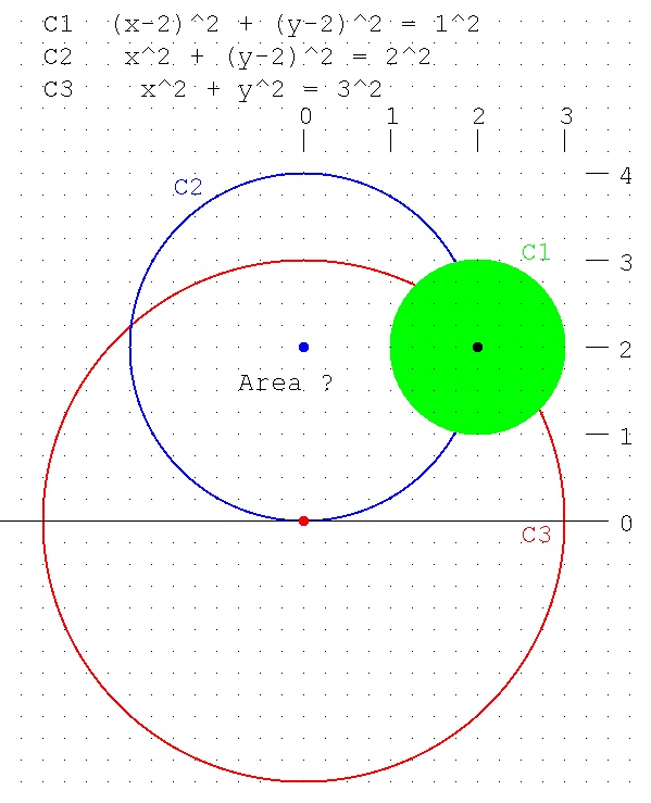
2. Write a small program in the language of your choice to
   numerically compute, to at least 3 significant digits,
   the area that is outside Circle 1 and inside both Circle 2
   and Circle 3,e.g. inside if x^2+y^2<9, outside if x^2+Y^2>9

   Circle 1 center at (2,2) radius 1   (x-2)^2+(y-2)^2=1^2
   Circle 2 center at (0,2) radius 2    x^2+(y-2)^2=2^2
   Circle 3 center at (0,0) radius 3    x^2+y^2=3^2

   Method: count the dots in the area and multiply count by the
   area of a square. Run with a grid 0.1, 0.01, and  0.001,
   print count of dots and area for each grid size,
   to see if your computation is converging. Obviously, if the
   left hand side of the equation is larger than the right
   hand side of the equation, the point is outside the circle.
   Obviously 0.1 is not exactly representable, thus "=" is useless.


submit cs455 hw3 your-source your-output    for 1a, 1b and 2

your-source  and  your-output  ust be  text files.
Do not submit  a.out  that is a binary file.


   (Note: in problem 2, if you were given a function z=F(x,y) and
    needed to compute the volume over the area, you would
    probably combine part of problem 1 with problem 2.)
Use a language and big numbers package of your choice to
compute the exact integer value of the following:

How many ways can you lay out a deck of cards in a line?
52 cards in a deck, all permutations is 52!.
Thus, just compute 52 factorial.

How many five card hands from a deck of 52 cards?
This is an n choose m problem. n! / ((n-m)! m!).
n is 52, m is 5. Direct computation, no math reductions.

print all digits as an integer, big number,
no scientific notation E+xx.

Turn in paper or submit cs455 hw4 your-source your-output.
(Clean out unused source code, it should be small.)
((Typically have a  fct(n) function in your code.))
See Lecture 19
last name a-j a, last name k-r b,  last name s-z c   ?
cp /afs/umbc.edu/users/s/q/squire/pub/download/q2_455a.doc
cp /afs/umbc.edu/users/s/q/squire/pub/download/q2_455b.doc
cp /afs/umbc.edu/users/s/q/squire/pub/download/q2_455c.doc

answer with libreoffice or Microsoft Word

submit cs455 quiz2 q2_455?.doc  or  q2_455?.docx
Use your browser to listen to  .wav  files.

you can use your browser to listen to files and to
copy files into your directory.
You and copy my files on gl.umbc.edu using:
cp  /afs/umbc.edu/users/s/q/squire/pub/download/xxx.wav .
for xxx= cat, short_count, train  etc.

Take a .wav file. Listen to it.
Extract the amplitude data from the .wav file.
Use a FFT to get the frequency spectrum.
Modify the frequency spectrum
Use inverse FFT to get amplitude data.
Insert the modified amplitude data into the .wav file.
Listen to the new .wav file.

Just do one of, a) b) c)

a) delete high and low frequencies from the spectrum or
   perform some other modification. Comment on how the
   sound changed.

b) Move all of the spectrum from i to n down into 1 to n-i,
   zero spectrum from n to top. You should be able to
   understand the modified .wav yet it will be a much
   deeper voice. You have lowered the frequency.

c) Mess up the sound with some other change to the spectrum.

Look at the spectrum plots. It depends on what code you use:
Possibly leave the zeroth frequency alone or zero it.
For N=2^n, leave the N/2 as it is, this is the Nyquist frequency.
Moving the top half down and the bottom half up, raises the pitch.
It also introduces noise.


Sample code for FFT and IFFT provided.
copy whatever you need from Lecture 18, FFT

Sample code to read and write a .wav is provided for a few languages.

waveplay.m reads a .wav file, plays the file
at three speeds, then writes a .dat file with just the sound.
The .dat file can be read with %f format. soundplay.m
Will play a .dat file, that may be read, modified, and rewritten.
In Matlab, if it works for you, use fft_wav.m

In Python, hack sound.py and use Python's fft and ifft.
Python sound may only work on Microsoft Windows.
UMBC screwed up Python, use your own computer and use
pip install on packages such as  wave  scipy  etc.
fftwav.py3 for fft and ifft on .wav


In Java, hack ClipPlayerTest.java and use
my Cxfft.java for fft and ifft functions.
There is read_wav.java to read
and write  .wav  files.
Or, if it works for you, use fft_wav.java
With a plot, use fft_frame.java

In Ubuntu using plain "C", hack pcm_dat.c and use any of the FFT and
IFFT written in "C".

The program read_wav.c reads and writes a .wav file.
You can put a FFT in between the read and write for your homework.
Use common existing software to play the .wav file(s).

You may need to convert complex values to magnitude.
Given a+bi  amplitude = sqrt(a*a+b*b)

Turn in paper or submit your source code,
submit input .wav files and output .wav files.

submit cs455 hw5 your-files

(option: use just ascii files of numbers, read and write with %f
 MatLab code  soundplay.m plays file.
 short_count.dat is one two three.)

See Lecture 18 for more information
Compile and run the program time_matmul.c
on some computer. You may use other languages and MatLab.
Time the matrix multiply for 100 by 100, 200 by 200, 400 by 400 etc
and record the actual time and a normalized time. It is OK to stop
when a single size takes over 10 minutes.

The normalized time is some constant multiplied by actual time divided by N^3.
Matrix multiply is order N cubed, thus the time goes up by a factor
of 8 each time N doubles. Note that the small 100 by 100 runs very fast.
As the matrix gets larger, the time increases by more than a factor of 8.
This is because of cache performance verses memory bandwidth.

If you can not run "C", a Java version, a little faster, is:
time_matmul.java

If you want a really slow version, run the Python:
time_matmul.py
Actually, you should be using  numpy  for numerical computation.
time_matmuln.py using numpy

Comment on or explain any large variation in normalized time,
normalized time should be the same for all sizes, for the
language and operating system and machine you ran this homework.

Turn in paper or submit your code (or my code) and your output and comment.

submit cs455 hw6 your-files
See Lecture 29
See Lecture 19
last name a-j a, last name k-r b,  last name s-z c   ?
cp /afs/umbc.edu/users/s/q/squire/pub/download/q3_455a.doc
cp /afs/umbc.edu/users/s/q/squire/pub/download/q3_455b.doc
cp /afs/umbc.edu/users/s/q/squire/pub/download/q3_455c.doc

answer with libreoffice or Microsoft Word

submit cs455 quiz3 q3_455?.doc  or  q3_455?.docx
Last updated 11/2/2021