[Robots Home] |
[Robots, Servo Info] |
[A Robot Project] |
[Robot Program]
[Robots Sensor] |
[My First Robot] |
[Other Robots] |
[Simulators]|
[Robot Control]
Robot Control
Computing commands for two wheel robot
Suppose you want to program an autonomous robot to go from
where it is to another location. If you have solved the
"localization problem" and know the coordinates and orientation
of where the robot is now, and know the coordinates and
orientation of where the robot is to go, then the following
program may be useful to you. The code is basic "C" code that
can be translated into any language of your choice. The
demonstration of the code uses OpenGL to display the movement
of a two wheeled robot. With some adaption the code can be
adapted to other types of robots.

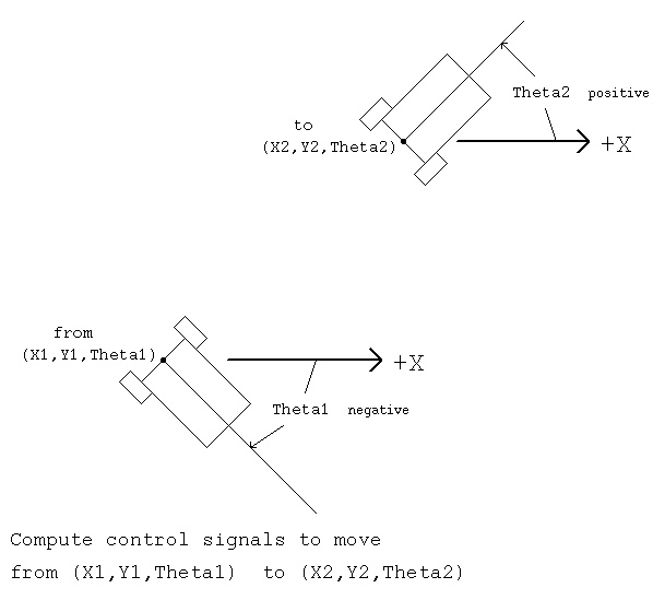
Given the current position of the robot as (X1, Y1, Theta1) and
the desired location (X2, Y2, Theta2) as shown below:


The problem is translated into a linear control system problem
where the goal is to reach the origin with the final direction
pointing along the positive axis as shown below:


The two figures show the geometry and definition of variables that
will be used to program the servo commands for a robot. The figures
are not related to each other.

The code, to be explained shortly, for linear control system command
computations is kine2r.c that uses
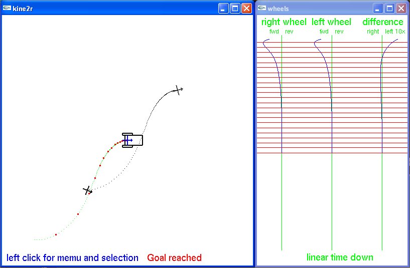
OpenGL to produce dynamic graphical output. A snap shot of the end
of one simulation is shown below.


The two wheel robot is at the "goal" (0,0) in control system coordinates.
The small + with arrow is the initial, lower, starting position in
world coordinates to upper final position in world coordinates.
The wheel rotation speeds and 10X difference are plotted on the right
with equal dt time steps.

A linear control system typically will be designed to drive all
dependent parameters to zero. This just simplifies the control
system. Thus, the initial calculation is to translate the destination
to coordinate (0,0) and rotate so that the destination angle is
zero degrees, pointing along the positive X axis.

The code could be:


  dx = x1-x2; /* translate destination to origin */
  dy = y1-y2;
  rho = sqrt(dx*dx+dy*dy); /* range to origin, which is "goal" */

  /* rotate to have destination be positive X axis */
  theta = theta1 - theta2;
  beta  = atan2(dy, dx);  /* angle robot center of wheels to goal */
  alpha = (-beta)-theta;  /* angle robot direction to goal */
  dx    = -dx; /* negate for control system equations */
  dy    = -dy;

  /* initialize
  t = 0.0;       /* time */

  /* prior analysis was used to determine control system */
  /* "gains" kr factor for rho, ka factor for alpha, kb factor for beta */

  /* compute deltas from control system */
  drho = -kr*rho*cos(alpha);
  dalpha = kr*sin(alpha) - ka*alpha - kb*beta;
  dbeta  = -kr*sin(alpha);
  dtheta = (-dbeta)-dalpha;

  /* control wants to move distance drho*dt */
  /*       at angle theta+dtheta*dt         */
  delx = drho*dt*cos(theta+dtheta*dt); /* change in dx */
  dely = drho*dt*sin(theta+dtheta*dt); /* change in dy */

  /* check if physical capability is exceeded         */
  /* effectively limit movement by using a smaller dt */
  del2S = 2.0*sqrt(delx*delx+dely*dely);
  delthetab = dtheta*dt*wwidth;
  delSr = (delthetab+del2S)/2.0;
  delSl = del2S-delSr;
  angright = -delSr/rwheel;
  angleft  = -delSl/rwheel;
  /* take into account radius of wheel and linear motion */
  /* to compute the commanded angle to move in time step dt */
  /* If physical limits are exceeded, limit the local */
  /* value of dt used in the following equations. */

  /* move the robot, dead reckoning, per control system path */
  dx = dx + delx;
  dy = dy + dely;
  rho = sqrt(dx*dx+dy*dy);
  theta = theta+dtheta*dt;
  alpha = -(theta - atan2(dy, dx));
  beta  = -(theta + alpha);
  t = t+dt; /* simulation time, or pseudo real time in the robot */


Reference: "Introduction to Autonomous Mobile Robots" by Siegwart
and Nourbakhsh. Section 3.6 pp 81-87, 5.2.4 P 187.


Some information on Kalman filter.
Last updated 4/20/05
 The problem is translated into a linear control system problem
where the goal is to reach the origin with the final direction
pointing along the positive axis as shown below:
 The two figures show the geometry and definition of variables that
will be used to program the servo commands for a robot. The figures
are not related to each other.
The code, to be explained shortly, for linear control system command
computations is kine2r.c that uses
OpenGL to produce dynamic graphical output. A snap shot of the end
of one simulation is shown below.
 The two wheel robot is at the "goal" (0,0) in control system coordinates.
The small + with arrow is the initial, lower, starting position in
world coordinates to upper final position in world coordinates.
The wheel rotation speeds and 10X difference are plotted on the right
with equal dt time steps.
A linear control system typically will be designed to drive all
dependent parameters to zero. This just simplifies the control
system. Thus, the initial calculation is to translate the destination
to coordinate (0,0) and rotate so that the destination angle is
zero degrees, pointing along the positive X axis.
The code could be:
dx = x1-x2; /* translate destination to origin */
dy = y1-y2;
rho = sqrt(dx*dx+dy*dy); /* range to origin, which is "goal" */
/* rotate to have destination be positive X axis */
theta = theta1 - theta2;
beta = atan2(dy, dx); /* angle robot center of wheels to goal */
alpha = (-beta)-theta; /* angle robot direction to goal */
dx = -dx; /* negate for control system equations */
dy = -dy;
/* initialize
t = 0.0; /* time */
/* prior analysis was used to determine control system */
/* "gains" kr factor for rho, ka factor for alpha, kb factor for beta */
/* compute deltas from control system */
drho = -kr*rho*cos(alpha);
dalpha = kr*sin(alpha) - ka*alpha - kb*beta;
dbeta = -kr*sin(alpha);
dtheta = (-dbeta)-dalpha;
/* control wants to move distance drho*dt */
/* at angle theta+dtheta*dt */
delx = drho*dt*cos(theta+dtheta*dt); /* change in dx */
dely = drho*dt*sin(theta+dtheta*dt); /* change in dy */
/* check if physical capability is exceeded */
/* effectively limit movement by using a smaller dt */
del2S = 2.0*sqrt(delx*delx+dely*dely);
delthetab = dtheta*dt*wwidth;
delSr = (delthetab+del2S)/2.0;
delSl = del2S-delSr;
angright = -delSr/rwheel;
angleft = -delSl/rwheel;
/* take into account radius of wheel and linear motion */
/* to compute the commanded angle to move in time step dt */
/* If physical limits are exceeded, limit the local */
/* value of dt used in the following equations. */
/* move the robot, dead reckoning, per control system path */
dx = dx + delx;
dy = dy + dely;
rho = sqrt(dx*dx+dy*dy);
theta = theta+dtheta*dt;
alpha = -(theta - atan2(dy, dx));
beta = -(theta + alpha);
t = t+dt; /* simulation time, or pseudo real time in the robot */
Reference: "Introduction to Autonomous Mobile Robots" by Siegwart
and Nourbakhsh. Section 3.6 pp 81-87, 5.2.4 P 187.
Some information on Kalman filter.