N. R. Miller
November 2000
Revided April 2004
2nd rev. June 2004
3rd rev. January
2006
4th rev. July 2006
HOW DOES THE ELECTORAL COLLEGE TRANSLATE POPULAR VOTES INTO ELECTORAL VOTES?
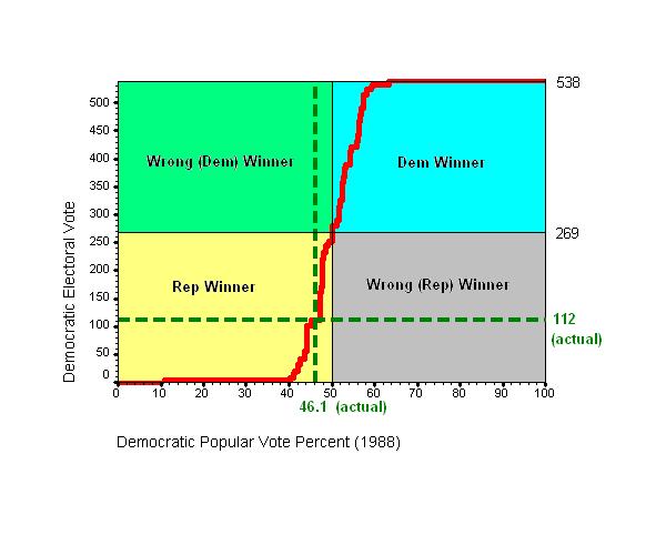
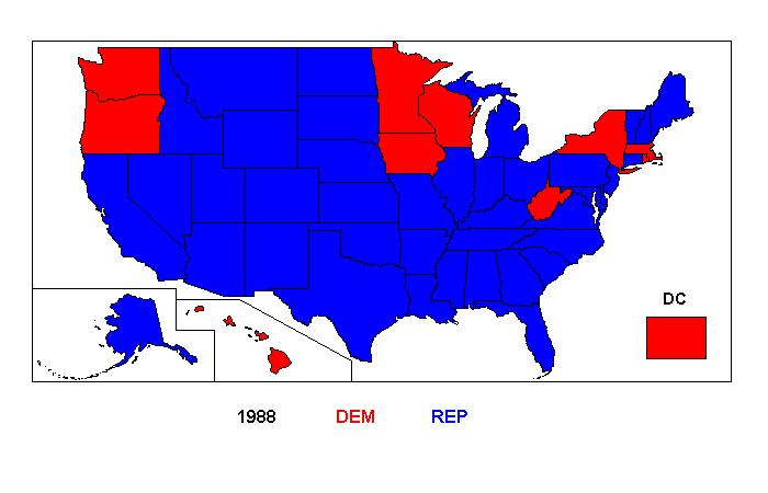
In the 1988 Presidential election, the Democratic ticket of Dukakis and Bentsen received 46.10% of the national popular vote and won 112 electoral votes (though one of these was lost to a “faithless elector”). Given state-by-state popular vote totals, we can display the relationship between Democratic popular and electoral votes in1988 by taking the actual state-by-state vote totals as the starting point and then considering how states would tip into or out the Democratic column in the face of a uniform national swing of varying magnitudes for or against the party. For example, a uniform national swing of 2.5% in favor of the Democrats would increase their national popular vote percent 46.1% to 48.6% and would shift every state they lost by less than 2.5% into the Democratic column.
Refer to this table.
(A) The
first column lists the states (plus DC) ordered in terms of the
performance of the Democratic ticket in the 1988 Presidential election.
(B) The next two
columns (DEM and REP) show the actual Democratic and Republican vote
for President (Presidential electors) in 1988.
(C) The fouth (D2PC) column shows the Democratic percent of the two-party presidential vote (i.e., DEM / (DEM + REP), thereby excluding votes casts for minor parties) in each state.
(D) The fifth column (DSWG) is equal to 50 - D2PC. Each negative entry represents the magnitude of a uniform national swing against the Democrats that would just cost them the state in question. For example, Dukakis carried his home state of MA with 53.98% of the 2-party vote. Thus Dukakis would still carry MA in the face of a uniform national swing against him of up to 3.98% but would lose it in the face of a larger national swing. Each positive entry represents the magnitude of a uniform national swing in favor of the Democrats that would just gain them the state in question. For example, Dukakis lost the megastate of CA with 48.19% of the vote. Thus Dukakis would still lose CA with a uniform national swing in his favor of anything less than 1.81% but would win with any larger favorable national swing.
(E) The sixth column (DPOP) is equal to 46.10 + DSWG. It represents the Democratic national popular vote resulting from a uniform national swing just big enough to tip the state. For example, the 3.98% national swing against the Democrats just sufficient to tip MA into the Republican column results in a 42.12% national popular vote for the Democrats; the 1.81% in favor of the Democrats just sufficient to tip CA into the Democratic column results in a 47.91% national popular vote for the Democrats.
(F) The fifth column (EVCM) is the total electoral vote for the Democratic ticket cumulating from their strongest to weakest state.
The fourth and
fifth columns together allow us to examine the relationship between
popular votes and electoral votes, taking the actual state-by-state
1988 vote as a baseline
and considering uniform national swings in both directions from this
baseline.
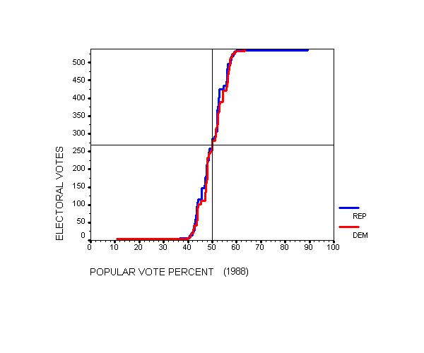
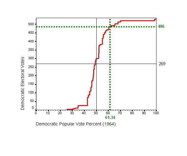
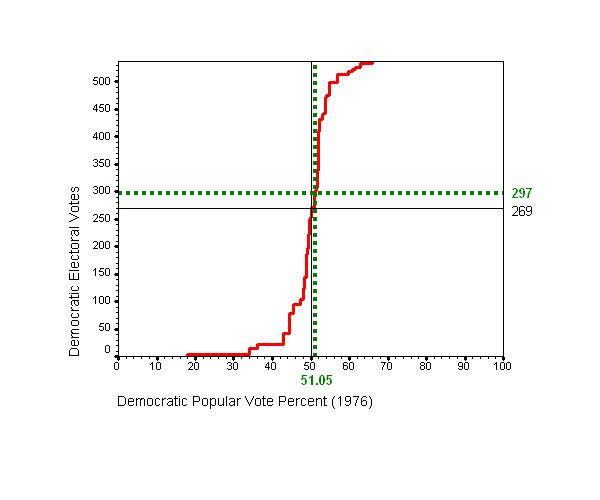
Plotting
EVCM against DPOP produces the monotonically increasing step function
shown in this
chart. The plot is monotonic because it assumes the increase
in the
Democratic national popular is uniform across states. It is a step
function because electoral
votes do not increase continuously with popular votes but rather in
discrete increments (of
no less than three votes) whenever another state tips into the
Democratic column. Dukakis
won 46.1% of the popular vote, which translated into 112 electoral
votes. This is shown in
the chart by the dashed green vertical and horizontal reference lines
that intersect at the
actual election outcome (DPOP = 46.1%, EVCM = 112). The table (and
less clearly the chart ) shows that (under the
uniform national swing assumption), if Dukakis had
won exactly 50.00% of the popular vote, he would have won 252 electoral
votes. It further shows that, if Dukakis had won anything less
than 50.08% of the national popular
vote (based on a uniform swing in his favor of about four percentage
points
in every state), he
would have won fewer than the 270 electoral votes required for election
but, once he hit
50.0765%, Michigan would have tipped into the Democratic column and
provided Dukakis
with a winning electoral vote total of 280. Thus 50.0765%
was the pivotal vote
percentage for Dukakis.
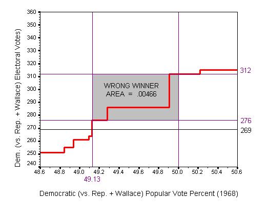
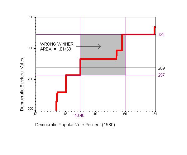
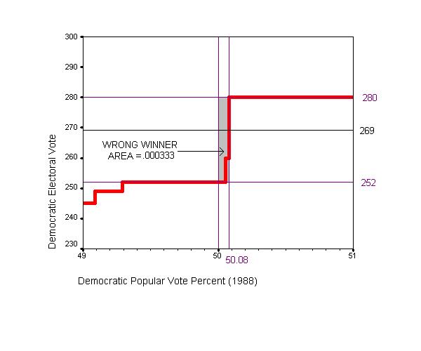
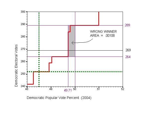
The chart is partitioned into four equal quadrants by the solid black vertical and horizontal reference lines located at DPOP = 50% and EVCUM = 269. An election outcome located at the intersection of these lines is a perfect tie, with respect to both popular and electoral votes. Any outcome (including the actual outcome) in the southwest quadrant (“Rep Winner”) is one in which the Democrats lose both the popular and electoral votes, while one in the northwest quadrant (“Dem Winner”) is one in which they win both the popular and electoral votes.
Assuming uniform national swings from the actual state-by-state popular vote, an Electoral College “wrong winner” (or “reversal of winners” or “misfire”) might have occurred given the 1988 baseline vote only if the plotted electoral vote function passes through either the northwest (“Wrong [Dem] Winner”) or southeast quadrants (“Wrong [Rep] Winner”) of the chart — which is to say, if fails to pass precisely through the perfect tie point at the center of the chart. (By monotonicity, the function can pass through at most one of the two wrong winner quadrants.) An outcome in the northwest quadrant entails a Democratic electoral vote victory with less than half of the two-party popular vote while an outcome in the southeast quadrant entail a Democratic electoral vote loss despite a popular vote majority. It is evident that, given any baseline vote, an electoral vote function will almost always fail to pass exactly through the precise center of the chart and that there is an essentially 50/50 chance that "wrong winner" may occur if the election is close enough with respect to electoral votes. In 1988 there would have been a “wrong winner” (under the uniform swing assumption) if Dukakis had received between 50.0000% and 50.0765% of the popular vote; given any larger swing in his favor, Dukakis would have carried Michigan and 280 electoral votes. The reversal of winners popular vote interval is about .0765 percentage points wide.
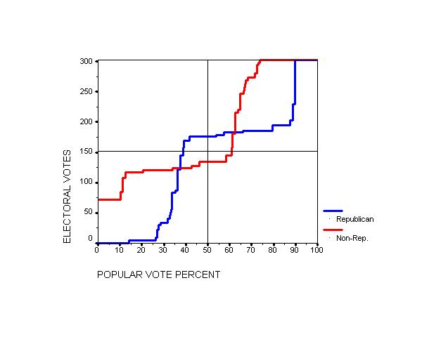
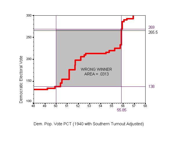
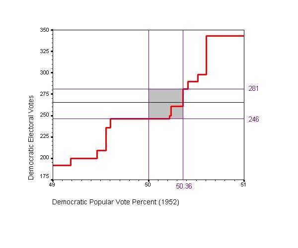
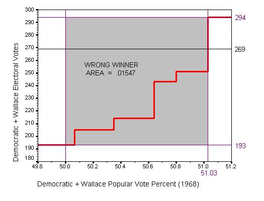
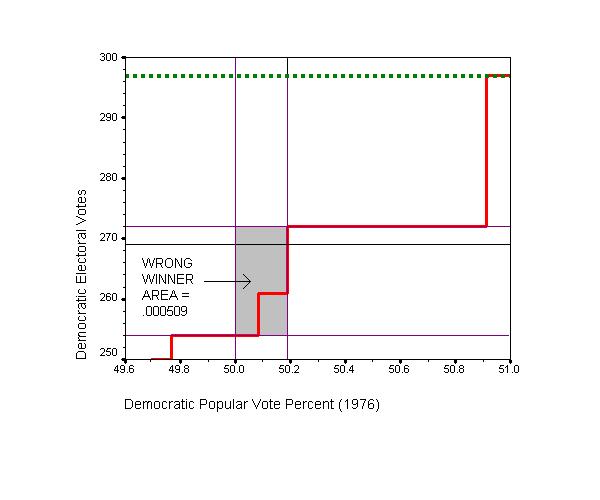
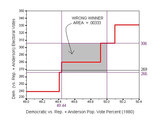
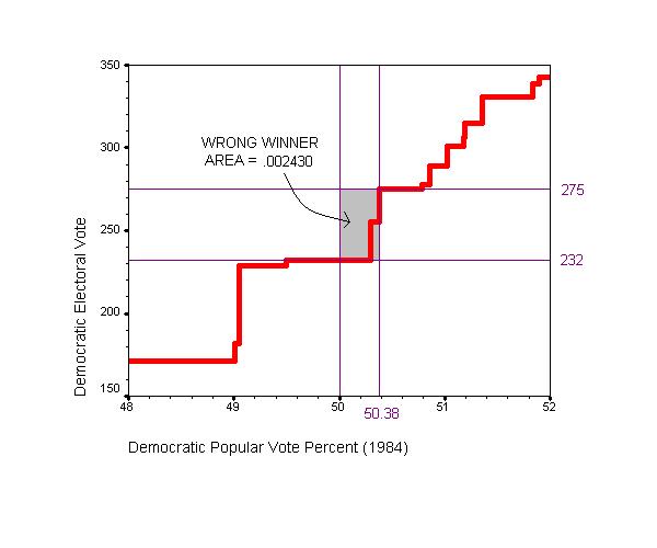
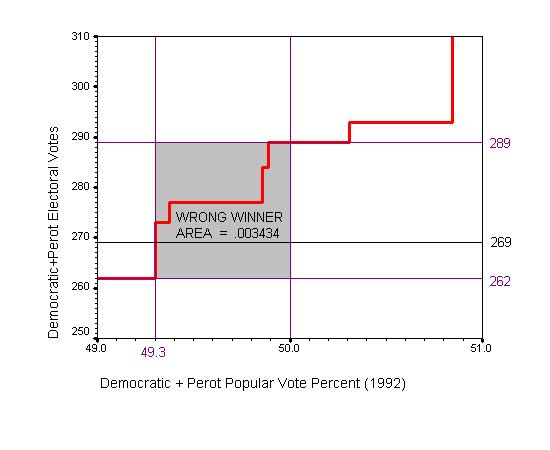
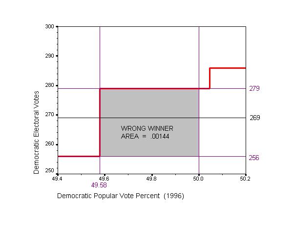
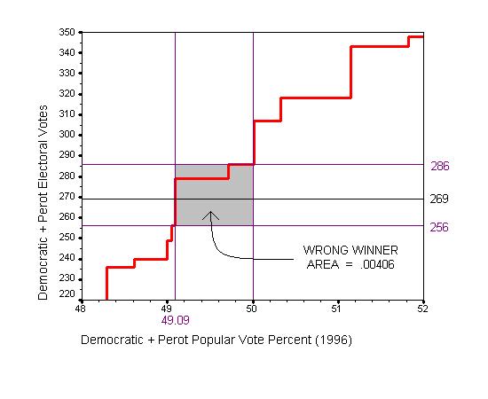
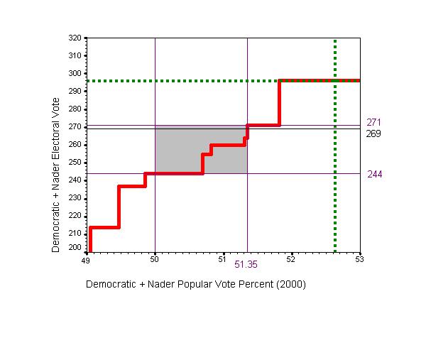
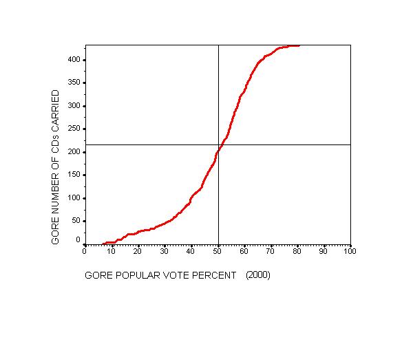
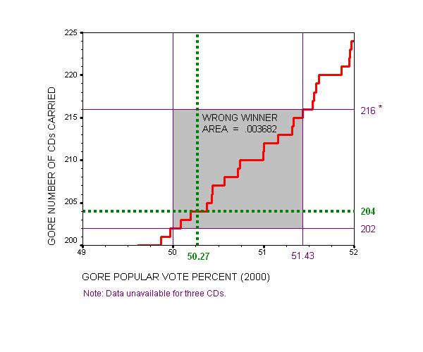
<> This chart zooms in on the critical region in the vicinity of DPOP = 50% to show the "wrong winner area” of the electoral vote function chart. This area is produced by multiplying the width of the wrong winner popular vote interval by the difference between electoral votes won at the the upper and lower bound of this interval. In the present case, this area is the rectangle with its southwest corner at 50% and 252 and its northwest corner at 50.0765% and 280. This rectangle occupies about .000037 of the total area in the full chart (i.e., 100% × 538) or about .000296 of the maximum wrong winner rectangle, which is deemed to be 12.5% of the full chart. The maximum wrong winner area occurs when a candidate receives a bare majority of popular votes in states with a bare majority of electoral votes and receives no popular votes in the remaining states (or, equivalently, when the other candidate falls ever so slightly behind in states with a bare majority of electoral votes and receives all the popular votes in the remaining states). In a perfect single-member district system with uniform turnout across districts, this means that one candidate wins a minimal majority of districts with just over 25% of the popular vote, while the other candidate wins a maximal minority of districts with just under 75% of the popular vote. This produces of maximum “wrong winner” rectangle region equal to one-eighth (12.5%) of the total area of the electoral vote function chart. (See this chart, in which 51% should really be read as 50+ε% and likewise for other percentages.)
This
visualization of the relationship between popular and electoral votes
makes
clear that there are two distinct ways in which a “wrong
winner” may occur.
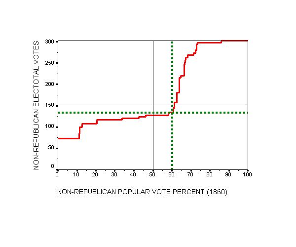
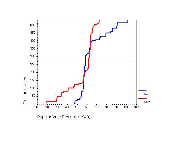
The grand daddy of all “wrong
winners” occurred in 1860, which exhibits the
same kind of bias as 1940 (and was also produced by extreme Republican
weakness in
the South) but
in even more extreme degree. It is well known that with slightly less
than 40% of the
national popular vote, Lincoln won a comfortable electoral vote
majority (180 out of 303)
against a divided opposition. But this victory was quite different
from, say, Wilson’s
electoral vote majority (435 out of 531) victory against a divided
opposition in 1912. Even
if he had confronted a single non-Republican candidate able to assemble
all Douglas,
Breckinridge, and Bell votes, Lincoln’s electoral vote total would have
been only slightly
reduced (whereas Wilson would have lost badly against a similarly
united opposition). The
only states that Lincoln actually won but would have lost against
united opposition were
California and Oregon (which he won by a pluralities against a divided
opposition). He
would have held every other state that he actually carried, because he
carried them with
an absolute majority of the popular vote. Though Douglas carried New
Jersey, Lincoln (for
peculiar reasons) won four of its seven electoral votes. Even if we
shift these four electoral
votes out of the Lincoln column along with the seven electoral votes
from California and
Oregon, Lincoln wins 169 electoral votes (with 39.8% of the popular
vote) against 134
electoral votes (with 60.2% of the popular vote) for the united
opposition. The 1860
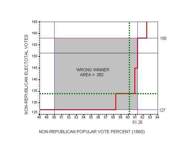
electoral vote function for this scenario is displayed in this chart
and this
zoom chart, in which the “wrong
winner” region occupies about .0922 of the potential space, over 300
times larger than in
1988.)
This possibility is clearly manifested by the 1988 chart, in which the electoral vote function exhibits no visible bias (at least in the critical region in the vicinity of DPOP = 50%). But as we saw in the earlier discussion of hypothetical uniform swing (and as was manifested in the actual outcome of the 2000 Presidential election), a "wrong winner" can occur in the absence of bias in the electoral vote function if the popular vote is extremely close.
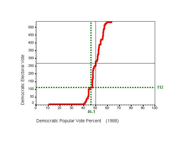
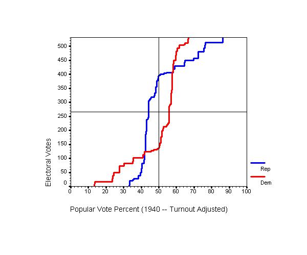
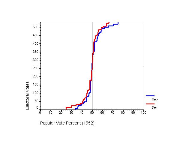
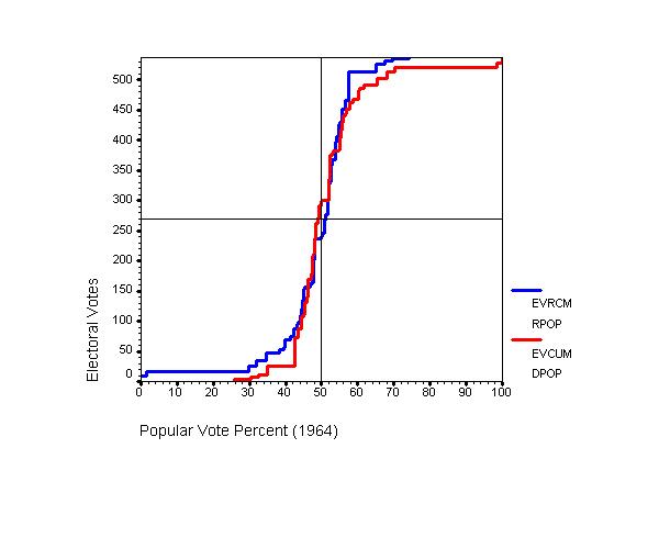
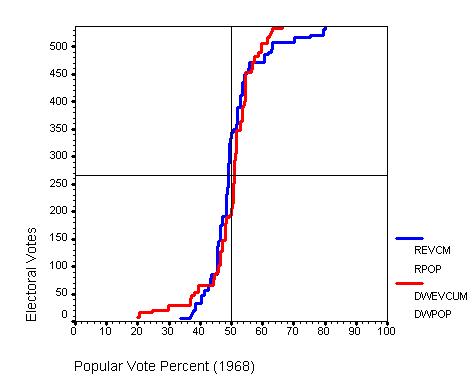
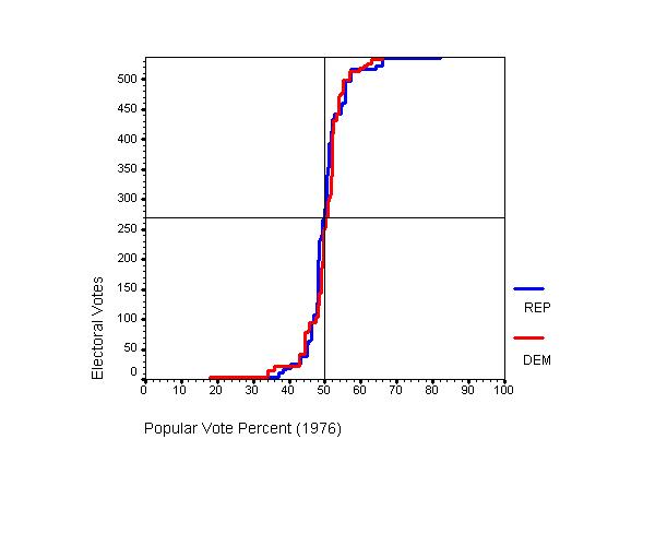
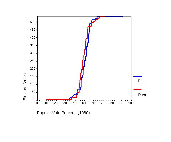
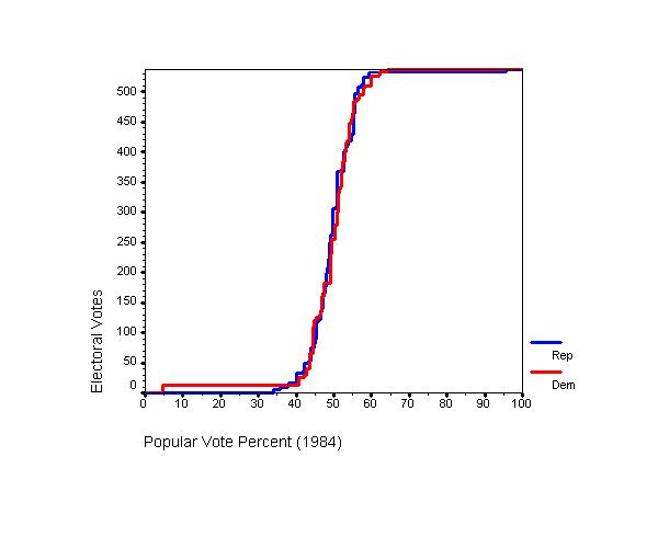
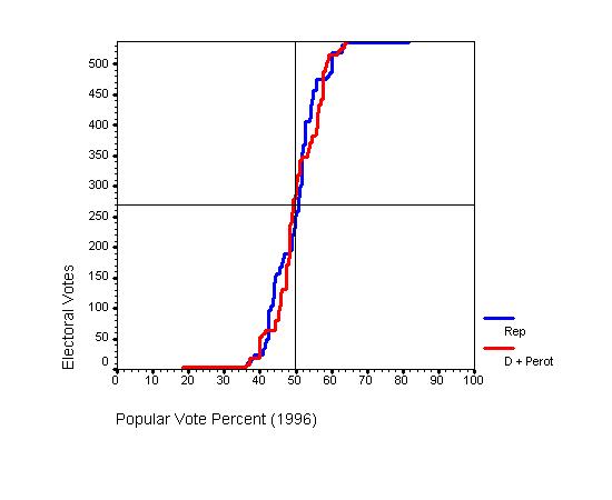
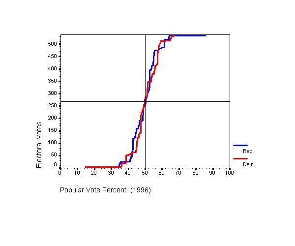
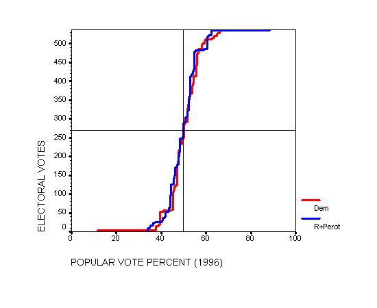
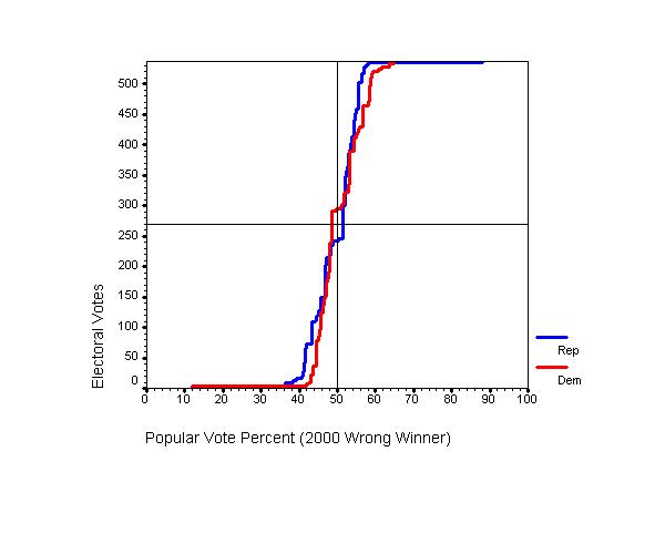
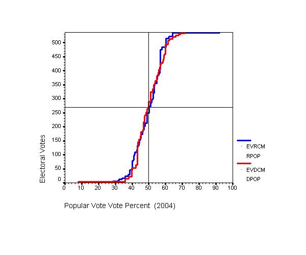
While it conveys no additional information, we can also construct a chart that superimposes the Republican electoral vote function on the Democratic electoral vote function and that makes evident any asymmetries between them when we look beyond the popular vote range close to 50%. It is evident that in 1988, there was no substantial asymmetry (despite talk on a Republican “electoral lock” on the Presidency).
The 1988 electoral vote function (like any typical two-party “votes/seats” curve) displays an S-shape, with the result that the curve is of maximum steepness in the vicinity of PV = 50%. Indeed, 1988 function is extremely steep in that vicinity. The steepness of such a function in the vicinity of 50% (say from 45% to 55%) is commonly called the swing ratio and expresses the magnitude of the impact of a uniform swing 1% of the popular vote on the resulting shift in the seat (or electoral vote) distribution, expressed as a percent of the seats (or electoral votes). The well-known “cube law” that seemed to operate in Britain in earlier times implies a swing ratio of about 3 — that is, if a party were to gain (or lose) 1% percent of the popular votes, it would be expected to gain (or lose) about 3% of the seats in the House of Commons. We can calculate the swing ratio for electoral votes by examining the electoral vote function between DPOP = 45% and DPOP = 55% and measuring its slope (i.e., the slope of the regression line fitted to this portion of the electoral vote function) when the vertical axis has been converted into percent of electoral votes, rather than number of electoral votes. In 1988, the swing ratio was an exceptionally high 6.3.
Charts similar to those for 1988 have been created for each Presidential election since 1828, as well as for other scenarios that result from pooling votes for minor and major candidates, which provides a basis for identifying “spoiler effects” of minor candidacies. Charts have also been created for scenario presented in Wrong Winner: The Coming Debacle in the Electoral College by David W. Abbott and James P. Levine. Note the wrong winner occurs because the electoral vote function has distinctive “shelf” built into it in the critical region that creates a substantial asymmetry in the electoral vote function. Nol electoral vote function based on actual popular vote data in a recent election exhibits such an asymmetry.
For
each election scenario, the following charts have been created:
LIST List of states, sorted by Democratic Popular Vote Percentage, showing
STATE:
State Postal Code
DEM Democratic
Popular Vote in the State
REP
Republican Popular Vote in the
State
D2PC: Democratic Percent of the 2-Party Popular Vote
DSWNG Swing from D2PC that would just tip the state into (positive swing) or out of (negative swing) the Democratic column
DPOP Democratic National Popular Vote Percent associated with DSWG (assuming swing is uniform across all states
EVCUM Cumulative Democratic Electoral Vote
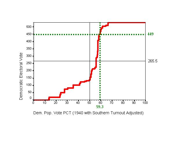
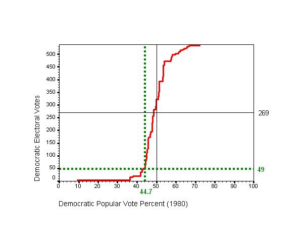
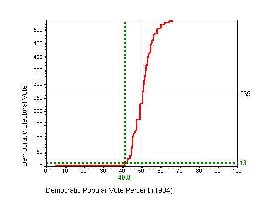
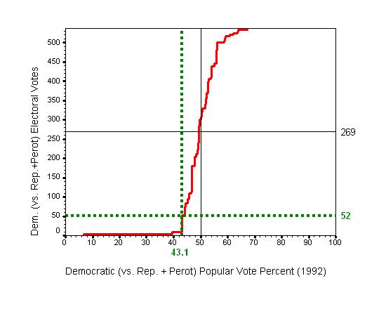
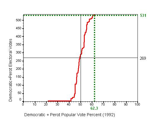
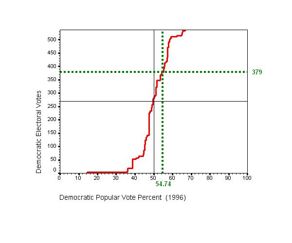
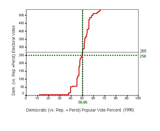
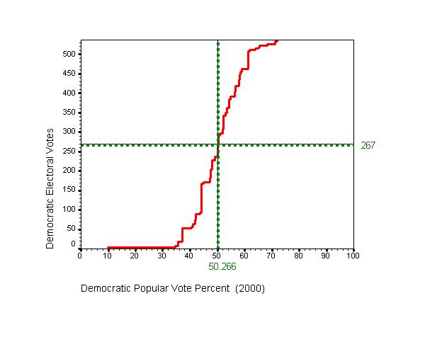
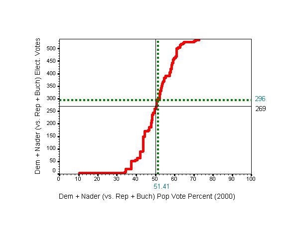
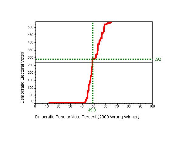
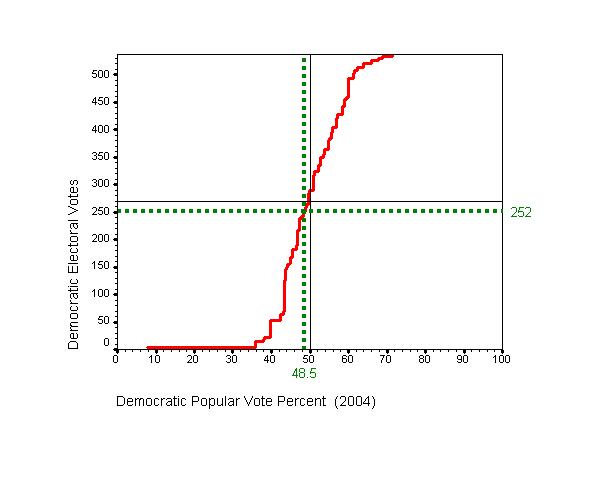
PVEV Electoral
Vote Function (the plot of EVCUM by DPOP), i.e., the translation
popular
votes into electoral votes, given the baseline or “landscape”
associated with D2PC. The actual Democratic popular vote
percent and electoral vote total is shown, as well the the electoral
vote that the Democratic candidate would have won with exactly 50.00%
of the national popular vote.
EVDR PVEV with corresponding Cumulative Republican Electoral Vote superimposed (to show any asymmetries/biases in the Electoral Vote Function)
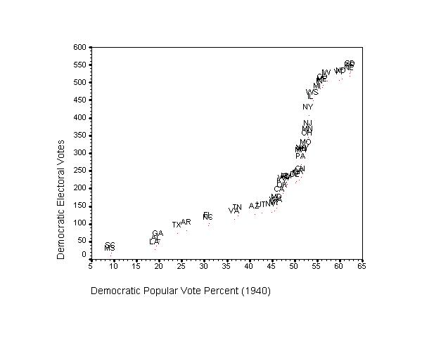
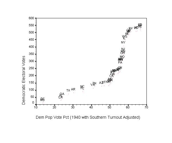
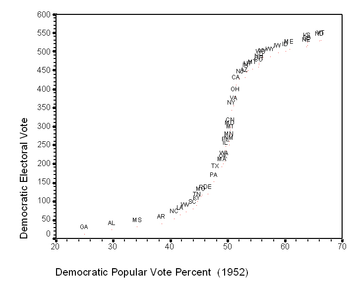
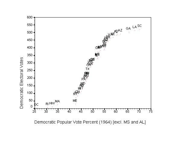
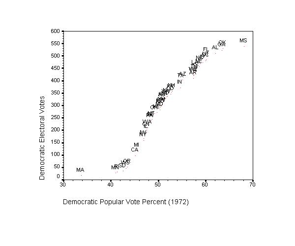
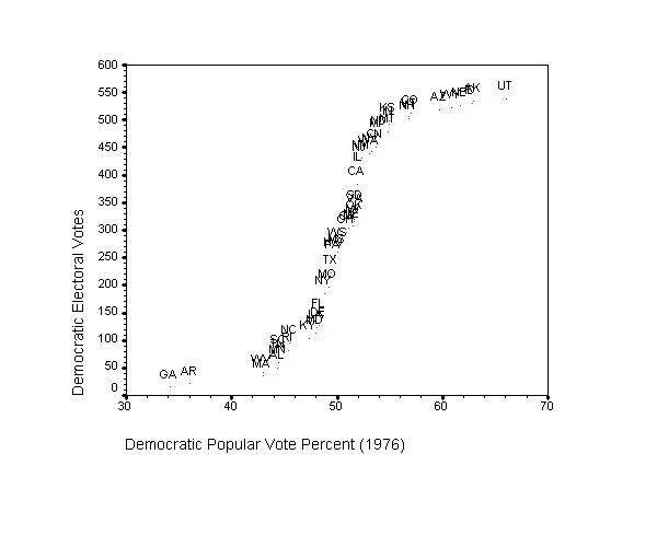
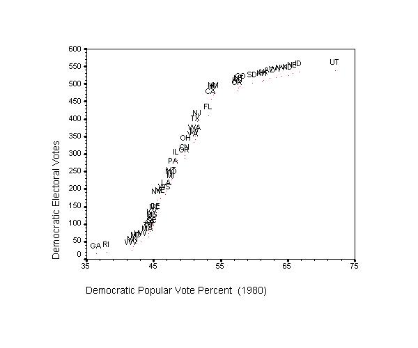
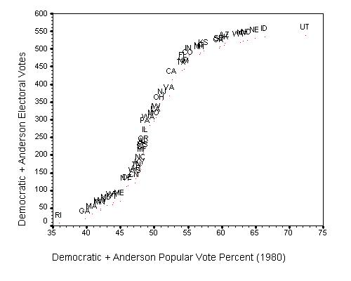
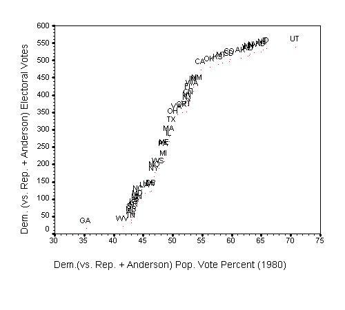
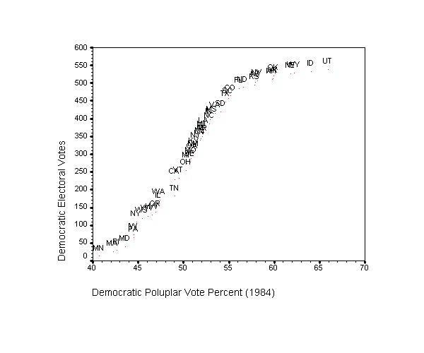
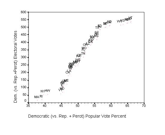
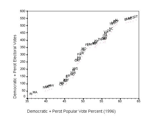
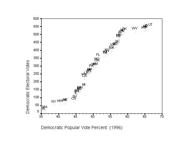
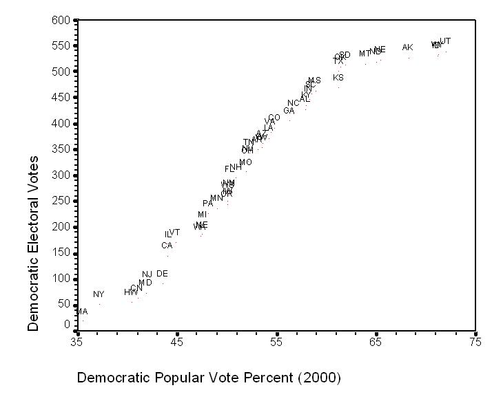
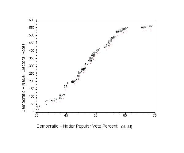
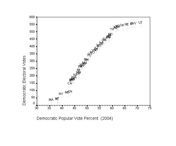
STATES Truncated version of PVEV without interpolation between points and with points identified by STATE code. (Note: each label appears slightly above the [almost invisible] plotted point.)
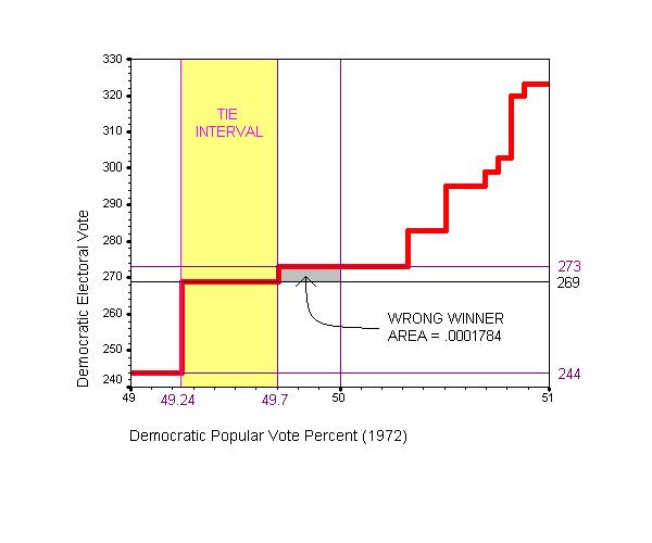
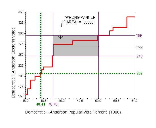
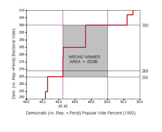
ZOOM A “zoom in” of PVEV at its center, i.e., in the vicinity of DPOP = 50% that
(i) identifies EVCUM for DPOP = 50% (i.e., the number of electoral votes the Democratic ticket would win when it gets just 50% of the popular vote);
(ii) identifies DPOP when EVCUM first constitutes a winning majority (270 at present); and
(iii) calculates the “wrong winner area,” i.e., the area of the rectangle shown in the zoom chart defined by the two points given by (i) and (ii), as a proportion of the maximum area (12.5%) of the PVEV chart that is logically subject to a possible “wrong winner.”
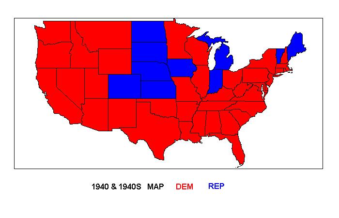
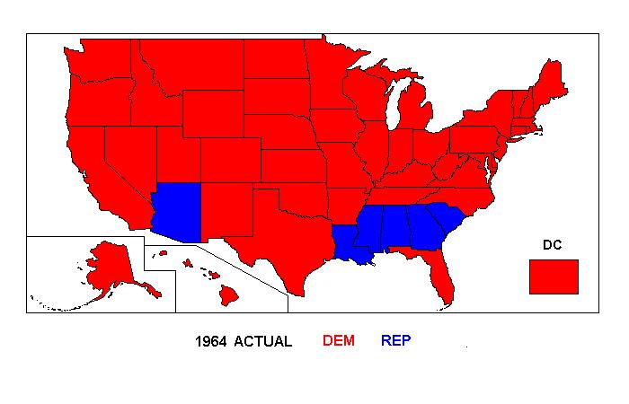
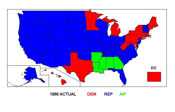
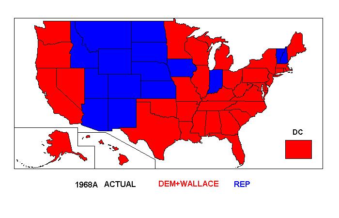
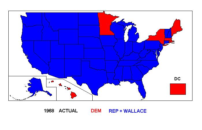
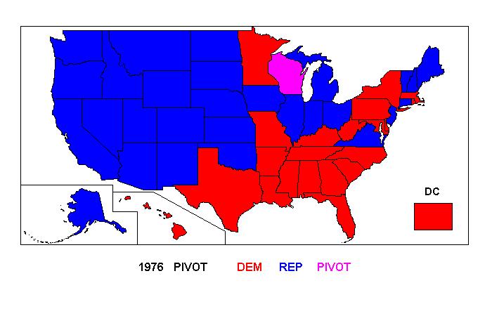
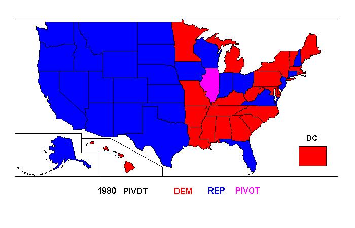
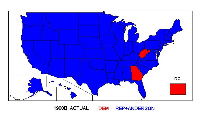
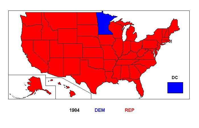
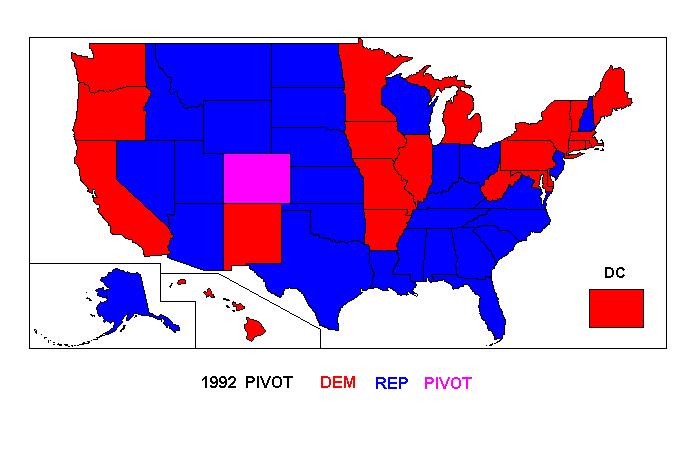
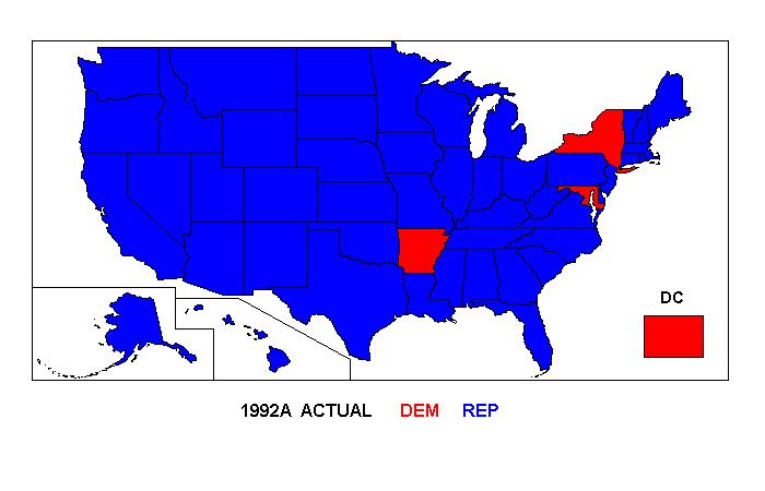
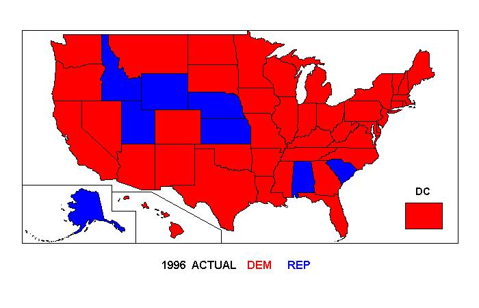
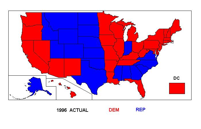
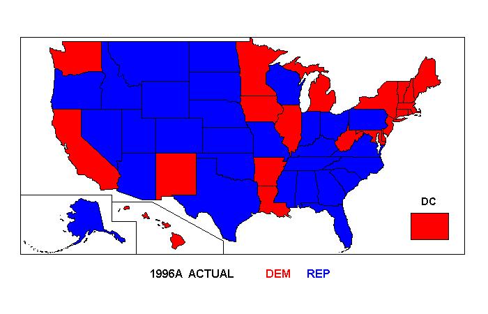
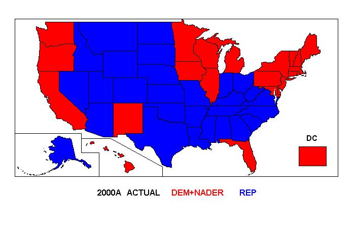
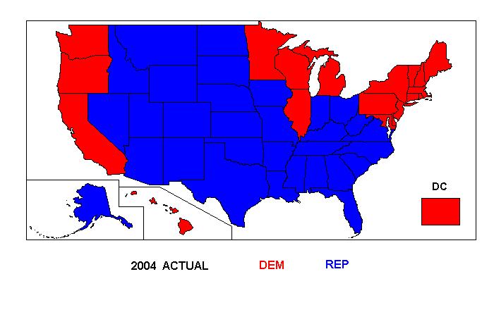
MAP The standard electoral vote map of the election outcome.
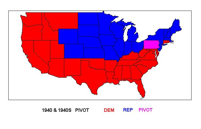
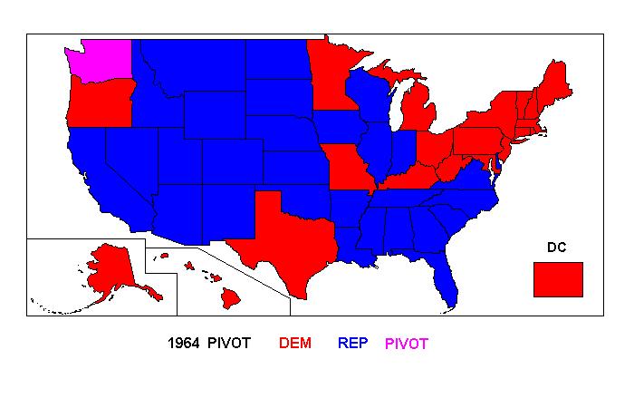
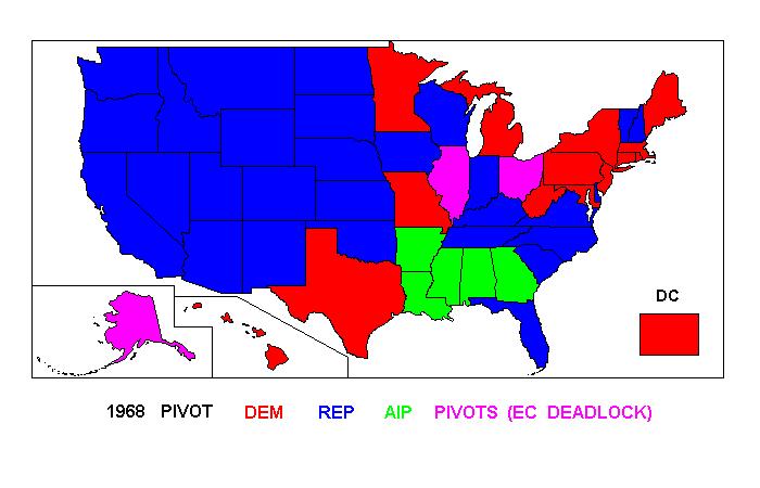
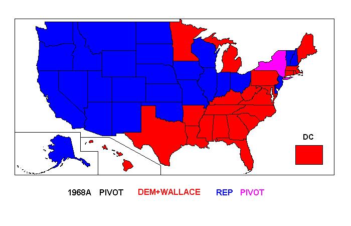
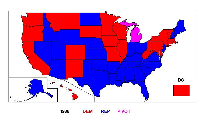
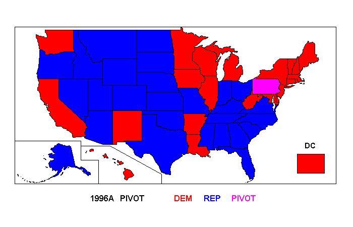
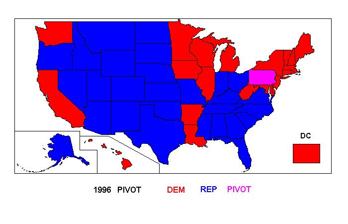
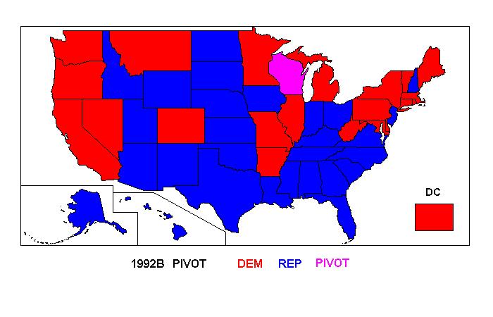
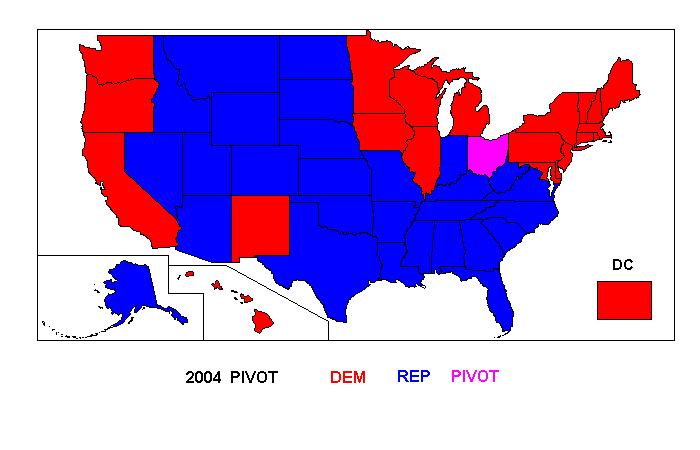
PIVOT An hypothetical electoral vote map that identifies the pivotal state on the LIST, together with the more Democratic and more Republican states. In effect, this is what the electoral map would have looked like (given the uniform swing assumption) in the closest possible electoral vote division that year (the winner being determined by the pivotal state).
PIVOT2 PIVOT with color tones showing relative party strength
PVEVS PVEV without Senatorial Bonus of 2 electoral votes for every state
PRESIDENTIAL ELECTION SCENARIOS
1828 Jackson
vs. Adams (Nat. Rep.) 1
1832X Jackson vs. Clay (Whig) 1
1832A Jackson vs. Clay (Whig) + Wirt (Anti-Masonic)
1836X Van Buren vs. Harrison + Webster + White (Whig) 2
1840 Van Buren vs. Harrison (Whig)
1844 Polk vs. Clay (Whig)
1848 Cass vs. Taylor (Whig)
1852 Pierce vs. Scott (Whig)
1852A Pierce vs. Scott (Whig) + Hale (Free Soil)
1856X Buchanan vs. Fremont (Rep.) 3
1856A Buchanan vs. Fremont (Rep.) + Fillmore (Whig-Am.)
1860A Douglas (N. Dem.) + Breckinridge (S. Dem.) + Bell (Const. U.) vs. Lincoln (Rep.)4
1860B Douglas (N. Dem.) + Breckinridge (S. Dem.) vs. Lincoln (Rep.)
1860C Douglas (N. Dem.) + Breckinridge (S. Dem.) vs. Lincoln (Rep.) + Bell (Const. U.)
1864 McClellan vs. Lincoln1868 Seymour vs. Grant
1872 Greely vs. Grant 5
1876 Tilden vs. Hayes
1880 Hancock vs. Garfield
1880A Hancock + Weaver (Greenback) vs. Garfield
1884 Cleveland vs. Blaine
1888 Cleveland vs. Harrison
1892X Cleveland vs. Harrison 6
1892A Cleveland + Weaver (Pop.) vs. Harrison
1892B Cleveland vs. Harrison + Weaver (Pop.)
1896 Bryan vs. McKinley
1900 Bryan vs. McKinley
1904 Parker vs. Roosevelt
1908 Bryan
vs. Taft
1912X Wilson vs. Taft 7
1912XX Wilson vs Roosevelt (Prog.) 8
1912A Wilson vs. Taft + Roosevelt (Prog.)
1912B Wilson
+ Roosevelt (Prog.) vs. Taft
1912C
Wilson + Debs (Soc.) vs. Taft + Roosevelt
(Prog.)
1916 Wilson vs. Hughes
1916A Wilson + Benson (Soc.) vs. Hughes
1920 Cox vs. Harding
1920A Cox + Debs (Soc.) vs. Harding
1924X Davis vs. Coolidge 9
1924A Davis + LaFollette (Prog.) vs. Coolidge
1924B Davis vs. Coolidge + LaFollette (Prog.)
1928 Smith vs. Hoover
1932 Roosevelt vs. Hoover
1936 Roosevelt vs. Landon
1940 Roosevelt vs. Willkie
1940S Roosevelt vs. Willkie (Southern turnout adjusted 10 )
1944 Roosevelt vs. Dewey
1948X Truman vs Dewey 11
1948A Truman + Thurmond (S.R Dem.) + Wallace (Prog.) vs. Dewey
1948B Truman + Wallace (Prog.) vs. Dewey + Thurmond (S.R Dem.)
1952 Stevenson vs. Eisenhower
1956 Stevenson vs. Eisenhower
1960X Kennedy vs. Nixon 12
1964 Johnson vs. Goldwater
1968X Humphrey vs. Nixon
1968A Humphrey + Wallace (AIP) vs. Nixon
1968B Humphrey vs. Nixon + Wallace (AIP)
1972 McGovern vs. Nixon
1976 Carter vs. Ford
1980 Carter vs. Reagan
1980A Carter + Anderson (Ind.) vs. Reagan
1980B Carter vs. Reagan + Anderson (Ind.)
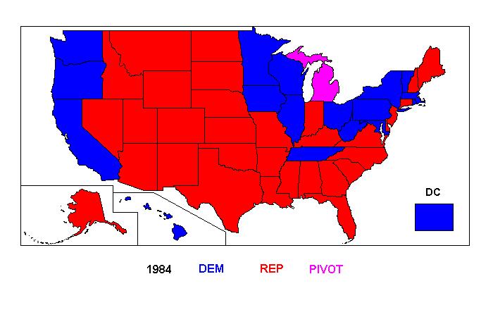
1984 Mondale vs. Reagan
1988 Dukakis vs. Bush
1992 Clinton vs. Bush
1992A Clinton vs. Bush + Perot (Ind.)
1992B Clinton + Perot (Ind.) vs. Bush
1996 Clinton vs. Dole
1996A Clinton vs. Dole + Perot (Reform)
1996B Clinton + Perot (Reform) vs. Dole
1996Z Clinton vs. Dole using Districted Electoral Vote System
2000 Gore vs. Bush
2000A Gore + Nader (Green) vs. Bush
2000B Gore vs. Bush + Buchanan (Reform)
2000C Gore
+ Nader (Green) vs. Bush + Buchanan (Reform)
2000CD
Gore vs. Bush
(based on Congressional Districts)
2000Z Gore vs. Bush using Districted Electoral Vote System
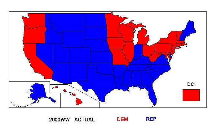
2000WW Bradley vs. Quayle (Wrong Winner) 13
2004 Kerry vs. Bush
Note 1. In elections in which a
third candidate wins electoral votes (by winning state-wide
pluralities), the basic chart applies the
uniform swing assumption to the Democratic vs. Republican candidate
contest, while holding the
third candidate's popular vote constant. As a result, some electoral
votes are
out-of-play and there are
three possible electoral vote outcomes: a Democratic majority, a
Republican majority, and an
Electoral College deadlock. Such charts are indicated as, for example,
1968X. Note that a
third candidate may fail to win a popular vote plurality in a state
but, if he wins more than one-third
of the popular vote in that
state, he would win a popular vote plurality (and the state’s electoral
votes) if the remaining votes
were sufficiently equally
divided between the Democratic and Republican candidates.
Conversely, a third candidate may win a popular popular vote plurality
(and the state's electoral votes) of less than 50% but would fail to do
so if
the remaining votes
were sufficiently unequally
divided between the Democratic and Republican candidates.
For example, in 1968 Wallace received 48% of the vote in Louisiana, 43%
in Georgia,
39% in Arkansas, and 34% in Tennessee, carrying all but TN (which Nixon
carried by a
plurality) by pluralities over both Humphrey and Nixon.
However, Humphrey or Nixon would have carried LA, GA, and AR given
large enough swinjgs in their favor (holding the Wallace vote
constant). On the other hand, a small swing towards
Humphrey would have tipped TN to Wallace (and a still
larger one would have tipped the state to Humphrey). Thus
the plot of the Wallace electoral vote by DPOP is an shallow
inverted U (see this chart).
Note 2. Since1828 onwards, electors have almost always been popularly elected on a general ticket (i.e., as a party slate). However, South Carolina electors were appointed by the legislature through 1860 and invariably cast all their votes for Democrats. (In 1832 and 1836, these electoral votes were cast for Democrats other than the national Democratic nominees; in these two years the South Carolina electoral votes are deemed to be out of play in the two-party analysis, so an EC deadlock might result.) In other years, the Democratic candidate is credited with the SC electoral votes from DPOP = 0 onwards. In 1868, the Florida legislature cast the states electoral votes (for Grant). In 1876, the Colorado legislature appointed its electors, which were cast for Hayes. In the analysis, Seymour and Tilden are not credited with the FL or CO electoral votes even at DPOP = 100.
Note 3. Because of the
general-ticket system for electing pledged electors, a state’s
electoral
are normally undivided. However, divisions in state electoral votes
occur in three circumstances:
(i) when electors violate their pledges (as a single elector has done
in each of these elections:
1956, 1960, 1968, 1972, 1976, 1988, and 2000); (ii) when electors are
elected at large but not
on a general ticket (as happened occasionally in the 19th
century and also in Alabama in 1960); and
(iii) when electors are elected from districts rather than statewide
(as happened in Michigan in 1892;
Nebraska and Maine have elected electors by district for several
elections but
this has never resulted in
a divide state electoral vote). At least one state split its electoral
votes (or an elector failed to vote) in each of the following
elections: 1828, 1832, 1860, 1864, 1872,
1880, 1892, 1896, 1904, 1908, 1912, 1916, 1948, 1956, 1960, 1968, 1972,
1976, 1988, and 2000. Since the
PVEV charts always credit the state
popular vote winner with
all the electoral votes
of the state, the electoral vote totals for candidates in these
elections differ slightly from the official record.
Notes on Inividual Elections
1828.
Maine, Maryland, and New York cast split electoral votes, with the
result that Jackson won 178 to 83 for Adams. As always, the
analysis credits the popular vote winner in a state with all of its
electoral votes.
1832.
Wirt
(Anti-Masonic) carried Vermont and was the only opposition to Clay in
Pennsylvania. Maryland split its electoral votes and failed
to cast two votes entirely, with the result that Jackson won 219
electoral votes to 49 for Clay, 11 (from SC; see Note 2) for Floyd, and
7 for Wirt.
3. Fremont received no more than a smattering of votes in any slave state, so Fillmore provided the only opposition to Buchanan in these states (and he actually carried Maryland).
4. Lincoln received no more than a smattering of votes in any slave state, and Douglas received few votes in the slave states. Breckinridge and Bell received few votes outside of the slave states. However, Breckinridge provided the main opposition to Lincoln in Pennsylvania. Lincoln received four of seven electoral votes from New Jersey, though Douglas carried the state. In the analysis, Douglas is credited with all seven electoral votes.
5. Greely died between the Presidential election and the casting of electoral votes. Congress refused to count three electoral votes cast for Greely himself; his electoral votes were scattered among four other candidates. Congress also refused to count the electoral votes of Arkansas and Louisiana (which Grant had carried), because of disruptive consitions during Reconstruction. In the analysis, this is treated as a normal two-party election with all electotal votes allocated on the basis of which party slate of electors carried the popular vote in each state.
6. Weaver carried Colorado, Idaho, Kansas, and Nevada. A number of states split their electoral votes. As always, the analysis credits all electoral votes to the popular vote winner in each state.
7. Theodore Roosevelt carried six states and received more than one-third of the vote in many others (and came in second in the national popular vote).
8. Taft carried two states and received more than one-third of the vote (and/or came in second) in many others.
9. LaFollete carried Wisconsin and received more than one-third of the vote is a number of states.
10. It
is assumed that the total popular vote of each southern state is equal
to that in a non-southern state with
the same number of electoral votes (the average of such states if there
are several or by interpolation if there
is none) and that this popular vote is divided between the candidates
in the same proportions as the actual
popular vote. This adjustment changes the electoral vote function but
does not affect the maps. Note that it is in effect assumed that
the additional popular votes in the South would have gone Democratic in
the same proportion as the votes actually cast. These additional
votes would have come mostly from disenfrachised blacks (plus some poor
whites), who probably would have voted heavily Democratic fro 1936
onwards, but the blacks at least would have voted heavily Republican
prior to the New Deal.
11. Thurmond
received no more than a smattering of votes outside of the South. He
carried Alabama, Mississippi, and South Carolina with with over 50% of
the vote and Louisiana with just under 50% but did not receive
one-third (or even one quarter) of the vote in any
state he did not carry. Wallace did not receive one quarter of
the
vote in any state. Truman was not
on the ballot in Alabama and could not receive any votes, so Alabama
must be excluded from uniform national swing calculations.
12. A slate of unpledged electors won a plurality of votes in Mississippi; however a Kennedy-pledged elector slate won more than one third of the votes. In Alabama, electors were elected statewide but not on a general ticket; moreover, six of the eleven Democratic electors (all of whom were elected) were unpledged. In the analysis, Kennedy is credited with the popular vote of the leading Kennedy-pledged elector and Nixon is credited with the popular vote of the leading Republican elector. However, Kennedy is credited with no more than the five electoral votes from Alabama that he actually won. The other six Alabama electoral votes, together with those of MS (while the Kennedy vs. Nixon vote is sufficiently close that the unpledged elector plurality is maintained), are considered to be out-of-play in the Kennedy-Nixon contest.
13. This is based on the scenario presented in Wrong Winner: The Coming Debacle in the Electoral College by David W. Abbott and James P. Levine. Note that the wrong winner occurs because the electoral vote function has a “shelf” built into it in the critical region near 50%. As can be checked, no actual electoral vote function in the present era has exhibited such a shelf.
1828 LIST PVEV EVDR STATES ZOOM MAP PIVOT PIVOT2 EVDRS
1832X LIST PVEV EVDR STATES ZOOM MAP PIVOT PIVOT2 EVDRS
1832A LIST PVEV EVDR STATES ZOOM MAP PIVOT PIVOT2 EVDRS
1836X LIST PVEV EVDR STATES ZOOM MAP PIVOT PIVOT2 EVDRS
1840 LIST PVEV EVDR STATES ZOOM MAP PIVOT PIVOT2 EVDRS
1844 LIST PVEV EVDR STATES ZOOM MAP PIVOT PIVOT2 EVDRS
1848 LIST PVEV EVDR STATES ZOOM MAP PIVOT PIVOT2 EVDRS
1852 LIST PVEV EVDR STATES ZOOM MAP PIVOT PIVOT2 EVDRS
1852A LIST PVEV EVDR STATES ZOOM MAP PIVOT PIVOT2 EVDRS
1856X LIST PVEV EVDR STATES ZOOM MAP PIVOT PIVOT2 EVDRS
1856A LIST PVEV EVDR STATES ZOOM MAP PIVOT PIVOT2 EVDRS
1860X LIST PVEV EVDR STATES ZOOM MAP PIVOT PIVOT2 EVDRS
1860A LIST PVEV EVDR STATES ZOOM MAP PIVOT PIVOT2 EVDRS
1860B LIST PVEV EVDR STATES ZOOM MAP PIVOT PIVOT2 EVDRS
1860C LIST PVEV EVDR STATES ZOOM MAP PIVOT PIVOT2 EVDRS
1864 LIST PVEV EVDR STATES ZOOM MAP PIVOT PIVOT2 EVDRS
1868 LIST PVEV EVDR STATES ZOOM MAP PIVOT PIVOT2 EVDRS
1872 LIST PVEV EVDR STATES ZOOM MAP PIVOT PIVOT2 EVDRS
1876 LIST PVEV EVDR STATES ZOOM MAP PIVOT PIVOT2 EVDRS
1880 LIST PVEV EVDR STATES ZOOM MAP PIVOT PIVOT2 EVDRS
1880A LIST PVEV EVDR STATES ZOOM MAP PIVOT PIVOT2 EVDRS
1884 LIST PVEV EVDR STATES ZOOM MAP PIVOT PIVOT2 EVDRS
1888 LIST PVEV EVDR STATES ZOOM MAP PIVOT PIVOT2 EVDRS
1892X LIST PVEV EVDR STATES ZOOM MAP PIVOT PIVOT2 EVDRS
1892A LIST PVEV EVDR STATES ZOOM MAP PIVOT PIVOT2 EVDRS
1892B LIST PVEV EVDR STATES ZOOM MAP PIVOT PIVOT2 EVDRS
1896 LIST PVEV EVDR STATES ZOOM MAP PIVOT PIVOT2 EVDRS
1900 LIST PVEV EVDR STATES ZOOM MAP PIVOT PIVOT2 EVDRS
1904 LIST PVEV EVDR STATES ZOOM MAP PIVOT PIVOT2 EVDRS
1908 LIST PVEV EVDR STATES ZOOM MAP PIVOT PIVOT2 EVDRS
1912X LIST PVEV EVDR STATES ZOOM MAP PIVOT PIVOT2 EVDRS
1912XX LIST PVEV EVDR STATES ZOOM MAP PIVOT PIVOT2 EVDRS
1912A LIST PVEV EVDR STATES ZOOM MAP PIVOT PIVOT2 EVDRS
1912B LIST PVEV EVDR STATES ZOOM MAP PIVOT PIVOT2 EVDRS
1916 LIST PVEV EVDR STATES ZOOM MAP PIVOT PIVOT2 EVDRS
1916A LIST PVEV EVDR STATES ZOOM MAP PIVOT PIVOT2 EVDRS
1920 LIST PVEV EVDR STATES ZOOM MAP PIVOT PIVOT2 EVDRS
1920A LIST PVEV EVDR STATES ZOOM MAP PIVOT PIVOT2 EVDRS
1924X LIST PVEV EVDR STATES ZOOM MAP PIVOT PIVOT2 EVDRS
1924A LIST PVEV EVDR STATES ZOOM MAP PIVOT PIVOT2 EVDRS
1928 LIST PVEV EVDR STATES ZOOM MAP PIVOT PIVOT2 EVDRS
1932 LIST PVEV EVDR STATES ZOOM MAP PIVOT PIVOT2 EVDRS
1936 LIST PVEV EVDR STATES ZOOM MAP PIVOT PIVOT2 EVDRS
1940 LIST PVEV EVDR STATES ZOOM MAP PIVOT PIVOT2 EVDRS
1940S LIST PVEV EVDR STATES ZOOM MAP PIVOT PIVOT2 EVDRS
1944 LIST PVEV EVDR STATES ZOOM MAP PIVOT PIVOT2 EVDRS
1948X LIST PVEV EVDR STATES ZOOM MAP PIVOT PIVOT2 EVDRS
1948A LIST PVEV EVDR STATES ZOOM MAP PIVOT PIVOT2 EVDRS
1948B LIST PVEV EVDR STATES ZOOM MAP PIVOT PIVOT2 EVDRS
1952 LIST PVEV EVDR STATES ZOOM MAP PIVOT PIVOT2 EVDRS
1956 LIST PVEV EVDR STATES ZOOM MAP PIVOT PIVOT2 EVDRS
1960X LIST PVEV EVDR STATES ZOOM MAP PIVOT PIVOT2 EVDRS
1964 LIST PVEV EVDR STATES ZOOM MAP PIVOT PIVOT2 EVDRS
1968X LIST PVEV EVDR STATES ZOOM MAP PIVOT PIVOT2 EVDRS
1968A LIST PVEV EVDR STATES ZOOM MAP PIVOT PIVOT2 EVDRS
1968B LIST PVEV EVDR STATES ZOOM MAP PIVOT PIVOT2 EVDRS
1972 LIST PVEV EVDR STATES ZOOM MAP PIVOT PIVOT2 EVDRS
1976 LIST PVEV EVDR STATES ZOOM MAP PIVOT PIVOT2 EVDRS
1980 LIST PVEV EVDR STATES ZOOM MAP PIVOT PIVOT2 EVDRS
1980A LIST PVEV EVDR STATES ZOOM MAP PIVOT PIVOT2 EVDRS
1980B LIST PVEV EVDR STATES ZOOM MAP PIVOT PIVOT2 EVDRS
1984 LIST PVEV EVDR STATES ZOOM MAP PIVOT PIVOT2 EVDRS
1988 LIST PVEV EVDR STATES ZOOM MAP PIVOT PIVOT2 EVDRS
1992 LIST PVEV EVDR STATES ZOOM MAP PIVOT PIVOT2 EVDRS
1992A LIST PVEV EVDR STATES ZOOM MAP PIVOT PIVOT2 EVDRS
1992B LIST PVEV EVDR STATES ZOOM MAP PIVOT PIVOT2 EVDRS
1996
LIST
PVEV EVDR STATES ZOOM MAP PIVOT PIVOT2 EVDRS
1996A
LIST PVEV EVDR STATES ZOOM MAP PIVOT PIVOT2 EVDRS
1996B
LIST PVEV EVDR STATES ZOOM MAP PIVOT PIVOT2 EVDRS
1996Z LIST PVEV EVDR STATES ZOOM MAP PIVOT PIVOT2 EVDRS
2000 LIST PVEV EVDR STATES ZOOM MAP PIVOT PIVOT2 EVDRS
2000A LIST PVEV EVDR STATES ZOOM MAP PIVOT PIVOT2 EVDRS
2000B LIST PVEV EVDR STATES ZOOM MAP PIVOT PIVOT2 EVDRS
2000C LIST PVEV EVDR STATES ZOOM MAP PIVOT PIVOT2 EVDRS
2000CD LIST
PVEV
EVDR STATES
ZOOM MAP
PIVOT
PIVOT2 EVDRS
2000Z LIST PVEV EVDR STATES ZOOM MAP PIVOT PIVOT2 EVDRS
2000WW LIST PVEV EVDR STATES ZOOM MAP PIVOT PIVOT2 EVDRS
2004 LIST PVEV EVDR STATES ZOOM MAP PIVOT PIVOT2 EVDRS
SUMMARY
TABLE: WRONG WINNER MARGINS AND SWING RATIOS