CS455 Selected Lecture Notes
This is one big WEB page, used for printing
 These are not intended to be complete lecture notes.
 Complicated figures or tables or formulas are included here
 in case they were not clear or not copied correctly in class.
 Computer commands, directory names and file names are included.
 Specific help may be included here yet not presented in class.
 Source code may be included in line or by a link.

 Lecture numbers correspond to the syllabus numbering.
Lecture 1, Introduction
Lecture 2, Rocket Science
Lecture 3, Simultaneous Equations
Lecture 3a, Case Study, Matrix Inversion
Lecture 3b, multiprocessors, MPI, threads and tasks
Lecture br, Boundary reduction of equations
Lecture 4, Least Square Fit
Lecture 5, Polynomials
Lecture 6, Curve Fitting
Lecture 7, Numerical Integration
Lecture 8, Numerical Integration 2
Lecture 9, Review 1
Lecture 10, Quiz 1
Lecture 11, Complex Arithmetic
Lecture 11, More Complex Arithmetic
Lecture 12, Complex Functions
Lecture 13, Eigenvalues of a Complex Matrix
Lecture 14, LAPACK
Lecture 15, Multiple precision, bignum
Lecture 16, Finding Roots and Nonlinear Equations
Lecture 17, Optimization, finding minima
Lecture 18, FFT, Fast Fourier Transform
Lecture 18a, Digital Filtering
Lecture 18b, Molecular frequency response
Lecture 19, Review 2
Lecture 20, Quiz 2
Lecture 21, Benchmarks, time and size
Lecture 22, Project Discussion
Lecture 23, Computing Volume and Area
Lecture 24, Numerical Differentiation
Lecture 24a, Computing partial derivatives
Lecture 24b, Computing partial derivatives in polar, cylindrical, spherical
Lecture 24b4, toward del^4 in spherical coordinates
Lecture 25, Ordinary Differential Equations
Lecture 26, Ordinary Differential Equations
Lecture 27, Partial Differential Equations
Lecture 27a, Differential Equation Definitions
Lecture ODE PDE Overview
Lecture 28, Partial Differential Equations
Lecture 28a, Additional Differential Equations
Lecture 28d, Biharmonic PDE using higher order
Lecture 28b, Navier Stokes case study
Lecture 28e, 5D five dimensions, independent variables
Lecture 28f, 6D six dimensions, Biharmonic
Lecture 28g, extended to 7 dimensions
Lecture 28k, extended to 8 dimensions
Lecture 28m, extended to 9 dimensions
Lecture 28h, PDE polar, cylindrical, spherical
Lecture 28j, PDE toroid geometry
Lecture 29, Review
Lecture 30, Final Exam
Supplemental L31, Creating PDE Test Cases
Supplemental L31a, sparse solution of PDE
Supplemental L31b, Nonlinear PDE
Supplemental L31c, Parallel PDE
Supplemental L31d, Parallel Multiple Precision PDE
Supplemental L32, Finite Element Method
Supplemental L33, Finite Element Method, triangle
Supplemental L33a, Lagrange fit triangle
Supplemental L34, Formats, reading
Lecture 28c, fem_50 case study
Supplemental L35, Navier Stokes Airfoil Simulation
Supplemental L36, Some special PDE's
Supplemental L36a, Special discretization, non uniform
Supplemental L37, Vaious utility
Supplemental L38, Open Tutorial on LaTeX
Supplemental L39, Tutorial on Numerical Solution of Differential Equations
Supplemental L40, Unique Numerical Solution of Differential Equations
Supplemental L41, Numerical solving AC circuits
Supplemental Airfoil lift and drag coefficients
Supplemental Continuum Hypothesis
openMP parallel computing
Supplemental Functional programming
Other Links
Introduction:
  Hello, my name is Jon Squire and I have been using computers
  to solve numerical problems since 1959. I have about 1 million
  lines of source code, in more than 15 languages,
  written over more than 50 years.
  How can that be? Check the numerical computation:
  1,000,000/50 years is 20,000 lines per year.
  20,000/200 working days per year is 100 lines per working day.
  Link to file type, file count, line count.

  With a lot of reuse, cut-and-paste, same programs and
  data files including scripts for many languages on many
  operating systems, easy.

  On a job, 20,000/(50 weeks*5 days per week) is 80 lines per day.
  80/8 hours is 10 lines per hour. You can do that.
  You may not save every line you type. sad.

Overview:
  You will be writing 6 small programs and a project in a language
  of your choice.
  Full details and sample code in a few lnguages will be provided.
  You will always have a weekend between a homework assignment
  and the due date.
  You may use whatever language or languages you like and you
  may experiment with other languages. Examples will be provided
  in C, Java, Python, Ruby, Matlab and others. You will see many
  languages including Fortran, Ada, Lisp, Pascal, Delphi, Scheme...
  The point is that the "syntactic sugar" of any language does
  not mean much. You may sometime convert code from some language
  into a language you like better.

  I have found some programs that I wrote can run faster in
  Java, Python, Ada, Fortran, Matlab than they run in optimized C.
  Well, the Python and Matlab use efficient library routines
  that are written in Fortran. We will cover threads and
  multiprocessor HPC concepts. There is a full course, CMSC 483
  Parallel and Distributed processing where you get to program
  a multiprocessor.

  You will be exposed to toolkits. Very valuable to help you
  produce more and better software with less effort. Over time
  you may develop a toolkit to help others. Toolkits are
  available for numerical computation, graphics, AI, robotics,
  any many other areas.

  Read the syllabus.


In this course there may be no exactly correct answer.

This lecture will provide the definitions and the intuition for
  absolute error
  relative error
  round off error
  truncation error

  Then how to call intrinsic function and elementary functions.

Some terms will be used without comment in the rest of the course.
Learn them now. You should run the sample code to increase your
understanding and belief.

"Absolute error" A positive number, the difference between the
exact (analytic) answer and the computed, approximate, answer.

"Relative error" A positive number, the Absolute Error divided
by the exact answer. (Not defined if the exact answer is zero.)

Most numerical software is first tested with one or more
known solutions. Then, the software may be used on
problems where the solution is not known.

Given the exact answer is 1000 and the computed answer is 1001:
The absolute error is 1
The relative error is 1/1000 = 0.001

For a set of computed numbers there are three common absolute errors:
"Maximum Error" the largest error in the set.
"Average Error" the sum of the absolute errors divided by the number
                in the set.
"RMS Error" the root mean square of the absolute errors.
            sqrt(sum_over_set(absolute_error^2)/number_in_set)

Given the exact answer is 100 answers of 1.0 and we
computed 99 answers of 1.0 and one answer of 101.0:
The maximum error is 100.0     101.0 - 1.0
The average error is 1.0       100.0/100
The RMS error is 10.0          sqrt(100.0*100.0/100)

In some problems the main concern is the maximum error, yet
the RMS error is often the best intuitive measure of error.
Generally much better intuitive measure than average error.

Almost all Numerical Computation arithmetic is performed using
IEEE 754-1985 Standard for Binary Floating-Point Arithmetic.
The two formats that we deal with in practice are the 32 bit and
64 bit formats. You need to know how to get the format you desire
in the language you are programming. Complex numbers use two values.

                                          older
        C       Java    Fortran 95        Fortran     Ada 95        MATLAB    Python R
        ------  ------  ----------------  ----------  ------------  --------  --------
32 bit  float   float   real              real        float         N/A       float
64 bit  double  double  double precision  real*8      long_float    'default' 'default'

complex
32 bit  'none'  'none'  complex           complex     complex       N/A       N/A
64 bit  'none'  'none'  double complex    complex*16  long_complex  'default' 'default'

'none' means not provided by the language (may be available as a library)
N/A means not available, you get the default.

IEEE Floating-Point numbers are stored as follows:
The single format 32 bit has
    1 bit for sign,  8 bits for exponent, 23 bits for fraction
                                          about 6 to 7 decimal digits
The double format 64 bit has
    1 bit for sign, 11 bits for exponent, 52 bits for fraction
                                          about 15 to 16 decimal digits

Some example numbers and their bit patterns:

   decimal
stored hexadecimal sign exponent  fraction                 significand

                                     The "1" is not stored |
                                                           |
                    31  30....23  22....................0  |
   1.0
3F 80 00 00          0  01111111  00000000000000000000000  1.0   * 2^(127-127)

   0.5
3F 00 00 00          0  01111110  00000000000000000000000  1.0   * 2^(126-127)

   0.75
3F 40 00 00          0  01111110  10000000000000000000000  1.1   * 2^(126-127)

   0.9999995
3F 7F FF FF          0  01111110  11111111111111111111111  1.1111* 2^(126-127)

   0.1
3D CC CC CD          0  01111011  10011001100110011001101  1.1001* 2^(123-127)


                          63  62...... 52  51 .....  0
   1.0
3F F0 00 00 00 00 00 00    0  01111111111  000 ... 000  1.0    * 2^(1023-1023)

   0.5
3F E0 00 00 00 00 00 00    0  01111111110  000 ... 000  1.0    * 2^(1022-1023)

   0.75
3F E8 00 00 00 00 00 00    0  01111111110  100 ... 000  1.1    * 2^(1022-1023)

   0.9999999999999995
3F EF FF FF FF FF FF FF    0  01111111110  111 ...      1.11111* 2^(1022-1023)

   0.1
3F B9 99 99 99 99 99 9A    0  01111111011  10011..1010  1.10011* 2^(1019-1023)
                                                                           |
                        sign   exponent      fraction                      |
                                                before storing subtract bias

Note that an integer in the range 0 to 2^23 -1 may be represented exactly.
Any power of two in the range -126 to +127 times such an integer may also
be represented exactly. Numbers such as 0.1, 0.3, 1.0/5.0, 1.0/9.0 are
represented approximately. 0.75 is 3/4 which is exact.
Some languages are careful to represent approximated numbers
accurate to plus or minus the least significant bit.
Other languages may be less accurate.

Now for some experiments for you to run an the computer of your choice
in the language of your choice.

In single precision floating point print:
    10^10 * sum( 1.0, 10^-7, -1.0)         answer should be  1,000
    10^10 * sum( 1.0, 0.5*10^-7, -1.0)     answer should be    500
    expression 10^10 * ( 1.0 + 10^-7 -1.0) answer should be  1,000
               10000000000.0*(1.0+10.0E-7-1.0)
The order of addition is important.
Adding a small number to 1.0 may not change the value.
This small number is less that what we call "epsilon".

error_demo1.adb Ada source code
error_demo1_ada.out output

error_demo1.c C source code
error_demo1_c.out output
epsilon.c C double and float source code
epsilon_c.out double and float output

error_demo1.f90 Fortran source code
error_demo1_f90.out output

error_demo1.java Java source code
error_demo1_java.out output

error_demo1.py3 Python source code
error_demo1_py3.out output

error_demo1.m Matlab source code
error_demo1_m.out output

error_demo1.r R source code
error_demo1_r.out output

Remember 10^-7 is 0.0000001, not a power of 2.
Thus, can not be stored exactly.
1.0e-16  = 10^-16 not exact because not a power of 2

Also, floating point arithmetic is performed in registers with
more bits than can be stored. Thus, as shown below, you may
get more precision than you expect. Do not count on it.
epsilon.c showing more precision source code
epsilon.out showing forced store output


We will cover, in the course,  methods of reducing error in areas:

statistics  sum x^2 - (sum x)^2  vs  sum(x-mean)

polynomial definition, evaluation Horner's rule vs x^N

approximation, e.g. sin(x)  truncation error vs roundoff error

derivatives

indefinite integral, definite integral, area

partial differential equations

and show sample code in many languages:
Ada 95, C, Fortran 95, Java, Python, MatLab and R

Error accumulation when computing standard deviation.
Subtracting large numbers loses significant digits.
 123456 - 123455 = 1.00000  only 1 significant digit
With only 6 digits representable
 123456.00 - 123455.99 = 1.00000 yet should be 0.010000


Two ways of computing the standard deviation are shown,
with the errors indicated for various sets of data:
Cases:
stddev(1, 2,..., 100)
stddev(10, 20,..., 1,000)              should just scale
stddev(100, 200,..., 10,000)
stddev(1,000, 2,000,..., 100,000)
stddev(10,000, 20,000,..., 1,000,000)
stddev(10,001, 10,002,..., 10,100)     should be same as first

See computed values in  .out  files:

sigma_error.c
sigma_error_c.out

sigma_error.f90
sigma_error_f90.out

sigma_error.adb
sigma_error_ada.out

sigma_error.java  float
sigma_error_java.out

sigma_errord.java  double
sigma_errord_java.out

sigma_error.py
sigma_error_py.out

sigma_error.m
sigma_error_m.out

Using different algorithms, expect slightly different results.
Using different types, float or double, may get very different results.

Iteration needing uniform step size should use multiplication,
not addition as shown in:
bad_roundoff.c
bad_roundoff_c.out


The elementary functions are sin, cos, tan, exp, sqrt
and inverse forms asin, acos, atan, log, power
and reciprocal forms cosecant, secant, cotangent,
and hyperbolic forms sinh, cosh, tanh,
and inverse hyperbolic forms asinh, acosh, atanh, ...

The intrinsic functions are built into the language, e.g. abs (sometimes)

Note that Fortran 95 and Java need no extra information to get the
real valued elementary functions. "C" needs #include <math.h>
while Ada 95 needs 'with' and 'use' Ada.Numerics.Elementary_functions .

Note that Ada 95 overloads the function names and provides
single precision as 'float' and double precision as 'long_float'.
ef_ada.adb Ada 95, float and long float

Note that Fortran 95, java, python, overload the function names and provides
the same function name for single and double precision.
Fortran 95 names single precision as 'real' and
double precision as 'double precision'.
ef_f95.f90 Fortran 95, real and double

Note that Java provides double precision as 'double' for variables and constants.
ef_java.java Java, only double
Hyper.java create your own hyperbolic

Note that C provides double precision only as 'double' and constants.
ef_c.c C, only double is available
ef_c.out nan means not a number, bad input

Note that MATLAB has the most functions and all functions are
automatically double or double complex as needed.
ef_matlab.m MATLAB everything
ef_matlab.out automatic complex

Note that Python needs  import math  and can list available functions
test_math.py Python many, automatic conversion
test_math_py.out Python output
test_math.py3 Python many, automatic conversion
test_math_py3.out Python output


Just for fun: Power of 2 "tree"

A small program that prints epsilon, 'eps' and the largest and
smallest floating point numbers, run on one machine, shows:

float_sig.c running, may die
type float has about six significant digits
eps is the smallest positive number added to 1.0f that changes 1.0f
type float eps= 5.960464478E-08
type float small= 1.401298464E-45
this could be about 1.0E-38, above shows un-normalized IEEE floating point
type float large= 1.701411835E+38

type double has about fifteen significant digits
type double eps= 1.11022302462515654E-16
type double small=4.940656458E-324
this could be about 1.0E-304, above shows un-normalized IEEE floating point
type double large=8.988465674E+307

The program is float_sig.c

Using 2^n = 10^k/3.32 and n bits has a largest number 2^n -1 and
k digits has a largest number 10^k -1. 24 bits would be 7 digits.
53 bits would be 16 digits, the more optimistic significant
digits for IEEE floating point.

Notes: I have chosen to keep most WEB pages plain text so that
they may be read by all browsers. Some referenced pages may
be .pdf, .jpg, .gif, .ps or other file types.
Many math books use many Greek letters. You may want to refer
to various alphabets.

If you want to stretch your concept of numbers,
check out the Continuum Hypothesis

Beware of easy methods of printing, related to epsilon
eps.py Python2 "print" Python3 "print( )"
eps.f90 Fortran "print"

You may use any language you want. I do not run your code.
Turn in paper in class or submit your source code and output for grading.
It is OK to ask for an example in a language I have not
provided. For various "C", I just provide .h and .c.
You may add to .h files for C++
  #ifdef __cplusplus
  extern "C" {
  #endif
  // header file function prototypes

  #ifdef __cplusplus
  }
  #endif

You may use Fortran and C object files in many
languages, including Java, Python, Matlab, etc.

Last updated 12/13/2021
Some physical problems are easy to solve numerically using just
the basic equations of physics. Other problems may be very difficult.
Consider a specific model rocket with a specific engine.
Given all the data we can find, compute the maximum altitude
the rocket can obtain. Yes, this is rocket science.
Most physics computation is performed with metric units.
units and equations
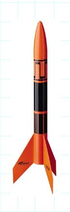 Estes Alpha III
Length 12.25 inches = 0.311 meters
Diameter 0.95 inches = 0.0241 meters
Body area 0.785 square inches = 0.506E-3 square meters cross section
Cd of body 0.45 dimensionless
Fins area 7.69 square inches = 0.00496 square meters total for 3 fins
Cd of fins 0.01 dimensionless
Weight/mass 1.2 ounce = 0.0340 kilogram without engine
Engine 0.85 ounce = 0.0242 kilogram initial engine mass
Engine 0.33 ounce = 0.0094 kilogram final engine mass
Estes Alpha III
Length 12.25 inches = 0.311 meters
Diameter 0.95 inches = 0.0241 meters
Body area 0.785 square inches = 0.506E-3 square meters cross section
Cd of body 0.45 dimensionless
Fins area 7.69 square inches = 0.00496 square meters total for 3 fins
Cd of fins 0.01 dimensionless
Weight/mass 1.2 ounce = 0.0340 kilogram without engine
Engine 0.85 ounce = 0.0242 kilogram initial engine mass
Engine 0.33 ounce = 0.0094 kilogram final engine mass
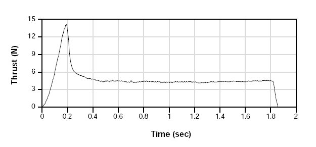 Thrust curve
Total impulse 8.82 newton seconds (area under curve)
Peak thrust 14.09 newton
Average thrust 4.74 newton
Burn time 1.86 second
Initial conditions:
t = 0 time
s = 0 height
v = 0 velocity
a = 0 acceleration
F = 0 total force not including gravity
m = 0.0340 + 0.0242 mass
i = 1 start with some thrust
Basic physics: (the order is needed for hw2)
(in while loop, start with time=0.1 thrust=6)
Fd = Cd*Rho*A*v^2 /2 two equations, body and fins
Fd is force of drag in newtons in opposite direction of velocity
Cd is coefficient of drag, dimensionless (depends on shape)
Rho is density of air, use 1.293 kilograms per meter cubed
A is total surface area in square meters
v is velocity in meters per second (v^2 is velocity squared)
Fg = m*g Fg is force of gravity toward center of Earth
m is mass in kilograms
g is acceleration due to gravity, 9.80665 meters per second squared
Ft = value from thrust curve array at this time, you enter this data.
index i, test i>18 and set Ft = 0.0 (time > 1.8 seconds)
Do not copy! This is part of modeling and simulation.
start with first non zero thrust.
F = Ft - (Fd body + Fd fins + Fg) resolve forces
a = F/m a is acceleration we will compute from knowing
F, total force in newtons and
m is mass in kilograms of body plus engine mass that changes
dv = a*dt dv is velocity change in meters per second in time dt
a is acceleration in meters per second squared
dt is delta time in seconds
v = v+dv v is new velocity after the dt time step
(v is positive upward, stop when v goes negative)
v+ is previous velocity prior to the dt time step
dv is velocity change in meters per second in time dt
ds = v*dt ds is distance in meters moved in time dt
v is velocity in meters per second
dt is delta time in seconds
s = s+ds s is new position after the dt time step
s+ is previous position prior to the dt time step
ds is distance in meters moved in time dt
m = m -0.0001644*Ft apply each time step
print t, s, v, a, m
t = t + dt time advances
i = i + 1
if v < 0 quit, else loop
Ft is zero at and beyond 1.9 seconds, rocket speed decreases
Homework Problem 1:
Write a small program to compute the maximum height when
the rocket is fired straight up. Assume no wind.
In order to get reasonable consistency of answers, use dt = 0.1 second
Every student will have a different answer.
Some where near 350 meters that is printed on the box. +/- 30%
Any two answers that are the same, get a zero.
Suggestion: Check the values you get from the thrust curve by
simple summation. Using zero thrust at t=0 and t=1.9 seconds, sampling
at 0.1 second intervals, you should get a sum of about 90 . Adjust
values to make it this value in order to get reasonable consistency of
answers.
The mass changes as the engine burns fuel and expels mass
at high velocity. Assume the engine mass decreases from 0.0242 kilograms
to 0.0094 grams proportional to thrust. Thus the engine mass is
decreased each 0.1 second by the thrust value at that time times
(0.0242-0.0094)/90.0 = 0.0001644 . mass=mass-0.0001644*thrust at this time.
"thrust" = 0.0 at time t=0.0 seconds
"thrust" = 6.0 at time t=0.1 seconds.
"thrust" = 0.0 at and after 1.9 seconds. Important, rocket is still climbing.
Check that the mass is correct at the end of the flight. 0.0340+0.0094
Published data estimates a height of 1100 feet, 335 meters to
1150 feet, 350 meters.
Your height will vary.
Your homework is to write a program that prints every 0.1 seconds:
the time in seconds
height in meters
velocity in meters per second
acceleration in meters per second squared
force in newtons
mass in kilograms (just numbers, all on one line)
and stop when the maximum height is reached.
Think about what you know. It should become clear that at each
time step you compute the body mass + engine mass, the three
forces combined into Ft-Fd_body-Fd_fins-Fg, the acceleration, the velocity
and finally the height. Obviously stop without printing if
the velocity goes negative (the rocket is coming down).
The program has performed numerical double integration. You might
ask "How accurate is the computation?"
Well, the data in the problem statement is plus or minus 5%.
We will see later that the computation contributed less error.
A small breeze would deflect the rocket from vertical and
easily cause a 30% error. We should say that:
"the program computed the approximate maximum height."
Additional cases you may wish to explore.
What is the approximate maximum height without any drag,
set Rho to 0.0 for a vacuum.
What is the approximate maximum height using dt = 0.05 seconds.
What is the approximate maximum height if launched at 45 degrees
rather than vertical, resolve forces in horizontal and vertical.
For this type of rocket to have stable flight the center of gravity
of the rocket must be ahead of the center of pressure. The center
of pressure is the centroid of the area looking at the side of
the rocket. This is why the fins extend out the back and the
engine mass is up in the rocket.
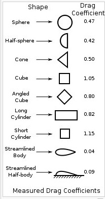
The shape of a moving object determines its drag coefficient, Cd.
The drag coefficient combined with velocity and area of the
moving object determine the drag force.
Fd = 1/2 * Cd * density * area * velocity^2
A few shapes and their respective drag coefficients are:
Thrust curve
Total impulse 8.82 newton seconds (area under curve)
Peak thrust 14.09 newton
Average thrust 4.74 newton
Burn time 1.86 second
Initial conditions:
t = 0 time
s = 0 height
v = 0 velocity
a = 0 acceleration
F = 0 total force not including gravity
m = 0.0340 + 0.0242 mass
i = 1 start with some thrust
Basic physics: (the order is needed for hw2)
(in while loop, start with time=0.1 thrust=6)
Fd = Cd*Rho*A*v^2 /2 two equations, body and fins
Fd is force of drag in newtons in opposite direction of velocity
Cd is coefficient of drag, dimensionless (depends on shape)
Rho is density of air, use 1.293 kilograms per meter cubed
A is total surface area in square meters
v is velocity in meters per second (v^2 is velocity squared)
Fg = m*g Fg is force of gravity toward center of Earth
m is mass in kilograms
g is acceleration due to gravity, 9.80665 meters per second squared
Ft = value from thrust curve array at this time, you enter this data.
index i, test i>18 and set Ft = 0.0 (time > 1.8 seconds)
Do not copy! This is part of modeling and simulation.
start with first non zero thrust.
F = Ft - (Fd body + Fd fins + Fg) resolve forces
a = F/m a is acceleration we will compute from knowing
F, total force in newtons and
m is mass in kilograms of body plus engine mass that changes
dv = a*dt dv is velocity change in meters per second in time dt
a is acceleration in meters per second squared
dt is delta time in seconds
v = v+dv v is new velocity after the dt time step
(v is positive upward, stop when v goes negative)
v+ is previous velocity prior to the dt time step
dv is velocity change in meters per second in time dt
ds = v*dt ds is distance in meters moved in time dt
v is velocity in meters per second
dt is delta time in seconds
s = s+ds s is new position after the dt time step
s+ is previous position prior to the dt time step
ds is distance in meters moved in time dt
m = m -0.0001644*Ft apply each time step
print t, s, v, a, m
t = t + dt time advances
i = i + 1
if v < 0 quit, else loop
Ft is zero at and beyond 1.9 seconds, rocket speed decreases
Homework Problem 1:
Write a small program to compute the maximum height when
the rocket is fired straight up. Assume no wind.
In order to get reasonable consistency of answers, use dt = 0.1 second
Every student will have a different answer.
Some where near 350 meters that is printed on the box. +/- 30%
Any two answers that are the same, get a zero.
Suggestion: Check the values you get from the thrust curve by
simple summation. Using zero thrust at t=0 and t=1.9 seconds, sampling
at 0.1 second intervals, you should get a sum of about 90 . Adjust
values to make it this value in order to get reasonable consistency of
answers.
The mass changes as the engine burns fuel and expels mass
at high velocity. Assume the engine mass decreases from 0.0242 kilograms
to 0.0094 grams proportional to thrust. Thus the engine mass is
decreased each 0.1 second by the thrust value at that time times
(0.0242-0.0094)/90.0 = 0.0001644 . mass=mass-0.0001644*thrust at this time.
"thrust" = 0.0 at time t=0.0 seconds
"thrust" = 6.0 at time t=0.1 seconds.
"thrust" = 0.0 at and after 1.9 seconds. Important, rocket is still climbing.
Check that the mass is correct at the end of the flight. 0.0340+0.0094
Published data estimates a height of 1100 feet, 335 meters to
1150 feet, 350 meters.
Your height will vary.
Your homework is to write a program that prints every 0.1 seconds:
the time in seconds
height in meters
velocity in meters per second
acceleration in meters per second squared
force in newtons
mass in kilograms (just numbers, all on one line)
and stop when the maximum height is reached.
Think about what you know. It should become clear that at each
time step you compute the body mass + engine mass, the three
forces combined into Ft-Fd_body-Fd_fins-Fg, the acceleration, the velocity
and finally the height. Obviously stop without printing if
the velocity goes negative (the rocket is coming down).
The program has performed numerical double integration. You might
ask "How accurate is the computation?"
Well, the data in the problem statement is plus or minus 5%.
We will see later that the computation contributed less error.
A small breeze would deflect the rocket from vertical and
easily cause a 30% error. We should say that:
"the program computed the approximate maximum height."
Additional cases you may wish to explore.
What is the approximate maximum height without any drag,
set Rho to 0.0 for a vacuum.
What is the approximate maximum height using dt = 0.05 seconds.
What is the approximate maximum height if launched at 45 degrees
rather than vertical, resolve forces in horizontal and vertical.
For this type of rocket to have stable flight the center of gravity
of the rocket must be ahead of the center of pressure. The center
of pressure is the centroid of the area looking at the side of
the rocket. This is why the fins extend out the back and the
engine mass is up in the rocket.
The shape of a moving object determines its drag coefficient, Cd.
The drag coefficient combined with velocity and area of the
moving object determine the drag force.
Fd = 1/2 * Cd * density * area * velocity^2
A few shapes and their respective drag coefficients are:
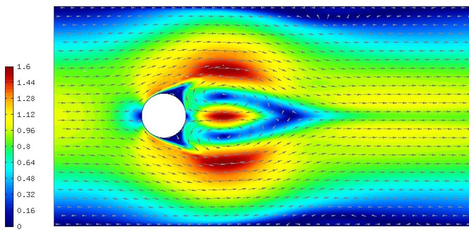
 We will cover numeric computation of flow.
 For more physics equations, units and conversion click here.
For more physics equations, center of mass, click here.
Homework 1 assignment
What you are doing is called "Modeling and Simulation", possibly
valuable buzz words on a job interview. Also "rocket scientist".
Observing what you are modeling may help.
For more physics equations, units and conversion click here.
For more physics equations, center of mass, click here.
Homework 1 assignment
What you are doing is called "Modeling and Simulation", possibly
valuable buzz words on a job interview. Also "rocket scientist".
Observing what you are modeling may help.
Simultaneous equations are multiple equations involving the same
variables. In general, to get a unique solution we need the
same number of equations as the number of unknown variables,
and the equations mutually linearly independent.
A sample set of three equations in three unknowns is:
eq1: 2*x + 3*y + 2*z = 13
eq2: 3*x + 2*y + 3*z = 17
eq3: 4*x - 2*y + 2*z = 12
One systematic solution method is called the Gauss-Jordan reduction.
We will reduce the three equations such that eq1: has only x,
eq2: has only y and eq3: has only z making the constant yield
the solution. Operations are always based on the latest version
of each equation. The numeric solution will perform the same
operations on a matrix.
Reduce the coefficient of x in the first equation to 1, dividing by 2
eq1: 1*x + 1.5*y + 1*z = 6.5
Eliminate the variable x from eq2: by subtracting eq2 coefficient of
x times eq1:
eq2: becomes eq2: - 3* eq1:
eq2: (3-3)*x + (2-4.5)*y + (3-3)*z = (17-19.5) then simplifying
eq2: 0*x - 2.5*y + 0*z = -2.5
Eliminate the variable x from eq3: by subtracting eq3 coefficient of
x times eq1:
eq3: becomes eq3: - 4* eq1:
eq3: (4-4)*x (-2 -6)*y + (2-4)*z = (12-26) then becomes
eq3: 0*x - 8*y - 2*z = -14
The three equations are now
eq1: 1*x + 1.5*y + 1*z = 6.5
eq2: 0*x - 2.5*y + 0*z = - 2.5
eq3: 0*x - 8.0*y - 2*z = -14.0
Reduce the coefficient of y in eq2: to 1, dividing by -2.5
eq2: 0*x + 1*y + 0*z = 1
Eliminate the variable y from eq1: by subtracting eq1 coefficient of y times eq2:
eq1: becomes eq1: -1.5* eq2:
eq1: 1*x + 0*y + 1*z = (6.5-1.5) then becomes
eq1: 1*x + 0*y + 1*z = 5
Eliminate the variable y from eq3: by subtracting eq3 coefficient of y times eq2:
eq3: becomes eq3: -8* eq2:
eq3: 0*x + 0*y - 2*z = (-14 +8) then becomes
eq3: 0*x + 0*y - 2*z = -6
The three equations are now
eq1: 1*x + 0*y + 1*z = 5
eq2: 0*x + 1*y + 0*z = 1
eq3: 0*x + 0*y - 2*z = -6
Reduce the coefficient of z in eq3: to 1, dividing by -2
eq3: 0*x + 0*y + 1*z = 3
Eliminate the variable z from eq1: by subtracting eq1 coefficient of z times eq2:
eq1: becomes eq1: -1* eq2:
eq1: 1*x + 0*y + 0*z = (5-3) then becomes
eq1: 1*x + 0*y + 0*z = 2
Eliminate the variable z from eq2: by subtracting eq2 coefficient of z times eq2:
eq2: becomes eq3: 0* eq2:
eq2: 0*x + 1*y + 0*z = 1
The three equations are now
eq1: 1*x + 0*y + 0*z = 2 or x = 2
eq2: 0*x + 1*y + 0*z = 1 or y = 1
eq3: 0*x + 0*y + 1*z = 3 or z = 3 the desired solution.
The numerical solution simply places the values in a matrix and uses the same
reductions shown above.
Given the equations: |A|*|X| = |Y| B = |AY|
eq1: 2*x + 3*y + 2*z = 13 | 2 3 2 | |x| |13|
eq2: 3*x + 2*y + 3*z = 17 | 3 2 3 |*|y|=|17|
eq3: 4*x - 2*y + 2*z = 12 | 4 -2 2 | |z| |12|
Create the matrix | 2 3 2 13 | having 3 rows and 4 columns
B = | 3 2 3 17 |
| 4 -2 2 12 |
The following code, using n=3 for these three equations, computes the
same desired solution as the manual method above.
for k=1:n
for j=k+1:n
B(k,j) = B(k,j)/B(k,k)
end
for i=1:n
if(i not k)
for j=1:n
B(i,j) = B(i,j) - B(i,k)*B(k,J)
Pivoting to avoid zero on diagonal and improve accuracy
Now we must consider the possible problem of B(k,k) being zero
for some value of k. It is rather obvious that the order of the
equations does not matter. The equations can be given in any
order and we get the same solution. Thus, simply interchange
any equation where we are about to divide by a zero B(k,k)
with some equation below that would not result in a zero B(k,k).
It turns out that we get better accuracy if we always pick
the equation that has the largest absolute value for B(k,k).
If the largest value turns out to be zero then there is no
unique solution for the set of equations.
We generally want numerical code to run efficiently and thus we
will not physically interchange the equations but rather keep
a row index array that tells us where the k th row is now.
The code for the final algorithm is given in the links below.
Note types of errors
test_simeq_small.c source code
test_simeq_small_c.out output
test_simeq_small.c results should be exactly X[0]=1.0, X[1]=-1.0
err is the error multiplying the solution, X, times matrix A*X=Y
a small change in data gives a big change in solution.
the big change is not indicated by the computed error.
decimal .835*X[0] + .667*X[1] = .168 Y[0]
decimal .333*X[0] + .266*X[1] = .067 Y[1]
flt-pt 0.835000*X[0] + 0.667000*X[1] = 0.168000
flt-pt 0.333000*X[0] + 0.266000*X[1] = 0.067000
initialization complete, solving
solution X[0]=1.0, err=0
solution X[1]=-1.0, err=0 -- expected
now perturb Y[1] from .067 to .066, .001 change, and run again
flt-pt 0.835000*X[0] + 0.667000*X[1] = 0.168000 Y[0]
flt-pt 0.333000*X[0] + 0.266000*X[1] = 0.066000 Y[1] -- only change
solution X[0]=-666.0, err=0
solution X[1]=834.0, err=2.84217e-14 -- X[1] WOW!
notice computed errors are still small,
yet, the values of X[0] and X[1] are very different.
Typical problem with people and computers:
Often called garbage in, garbage out!
test_inverse_small.c source code
test_inverse_small_c.out output
We will see later, when the norm of the coefficients of
simultaneous equations is inverted, and the norm of the inverse
is different by many orders of magnitude, the system will be
called ill-conditioned.
solving for function values on a grid
Solving for unknown function values on a given x,y grid:
test_eqn1 2*U(x,y) = C(x,y)
test_eqn2 2*U(x,y) + 3*V(x,y) = C(x,y)
3*U(x,y) + 3*V(x,y) = D(x,y)
test eqn3 2*U(x,y) + 3*V(x,y) + 4*W(x,y) = C(x,y)
4*U(x,y) + 2*V(x,y) + 3*W(x,y) = D(x,y)
3*U(x,y) + 4*V(x,y) + 2*W(x,y) = E(x,y)
test_eqn1.java source code
test_eqn1_java.out source code
test_eqn2.java source code
test_eqn2_java.out source code
test_eqn3.java source code
test_eqn3_java.out source code
test_eqn33.java source code
test_eqn33_java.out source code
test_eqn1.py3 source code
test_eqn1_py3.out source code
test_eqn2.py3 source code
test_eqn2_py3.out source code
test_eqn3.py3 source code
test_eqn3_py3.out source code
test_eqn33.py3 source code
test_eqn33_py3.out source code
Later lecture covers non linear equations.
Working code in many languages
The instructor understands that some students have a strong
prejudice in favor of, or against, some programming languages.
After about 50 years of programming in about 50 programming
languages, the instructor finds that the difference between
programming languages is mostly syntactic sugar. Yet, since
students may be able to read some programming languages
easier than others, these examples are presented in "C",
Fortran 95, Java and Ada 95. The intent was to do a quick
translation, keeping most of the source code the same,
for the different languages. Style was not a consideration.
Some rearranging of the order was used when convenient.
The numerical results are almost exactly the same.
The same code has been programmed in "C", Fortran 95, Java and Ada 95 etc.
as shown below with file types .c, .f90, .java and .adb .rb .py .scala:
Note the .h for C offers the user choices.
simeq.c "C" language source code
simeq.h "C" header file
time_simeq.c "C" language source code
time_simeq.out output
simeq.f90 Fortran 95 source code
time_simeq.f90 Fortran 95 source code
time_simeq_f90_cs.out output
simeq.java Java source code
time_simeq.java Java source code
time_simeq_java.out output
simeq.cpp C++ language source code
simeq.hpp C++ header file
test_simeq.cpp C++ language source code
test_simeq_cpp.out output
simeq.adb Ada 95 source code
real_arrays.ads Ada 95 source code
real_arrays.adb Ada 95 source code
Simeq.rb Ruby class Simeq
test_simeq.rb Ruby source code
test_simeq_rb.out Ruby output
simeq in matrix.pm Perl package
test_matrix.pl Perl source code test
test_matrix_pl.out Perl output
simeq.m MATLAB source code
simeq_m.out MATLAB output
With Python and downloading numpy using linalg
test_solve.py Python source code
test_solve_py.out Python output
With Python using numpy and array
test_simeq.py Python source code
test_simeq_py.out Python output
test_simeq.py3 Python source code
test_simeq_py3.out Python output
test_matmul.py3 Python source code
test_matmul_py3.out Python output
With Scala using Random, very small errors
Simeq.scala Scala source code
TestSimeq.scala Scala source code
TestSimeq_scala.out Scala output
Many methods have been devised for solving simultaneous equations.
A sample is LU decomposition and Crout method.
LU decomposition with pivoting:
lup_decomp.f90 source code
lup_decomp_f90.out output
simeq_lup.h source code
simeq_lup.c source code
time_simeq_lup.c source code
time_simeq_lup_cs.out output
simeq_lup.java source code
time_simeq_lup.java source code
time_simeq_lup_java.out output
Crout method without pivoting, uses back substitution:
crout.adb source code
crout_ada.out output
crout.f90 source code
time_crout.f90 source code
time_crout_f90.out output
crout.h source code
crout.c source code
time_crout.c source code
time_crout.c source code
time_crout_c.out output
crout1.h source code
crout1.c source code
time_crout1.c source code
time_crout1_c.out output
crout.java source code
test_crout.java accuracy test source
test_crout_java.out output
crout1.java source code
time_crout.java accuracy test source
time_crout_java.out output
Back substitution:
The difference from plain Gauss-Jordan with pivoting
and back substitution is less inner reduction,
then use back substitution. Solve A * X = Y
The initial reduction creates a matrix of the form:
| 1 a12 a13 a14 y1 |
| 0 1 a23 a24 y2 |
| 0 0 1 a34 y3 |
| 0 0 0 1 y4 |
Thus we have x4 = y4
Back substituting x3 = y3 - x4*a34
Back substituting x2 = y2 - x3*a23 - x4*a24
Back substituting x1 = y1 - x2*a12 - x3*a13 - x4*a14
simeq_back.h source code
simeq_back.c source code
test_simeq_back.c source code
test_simeq_back.out output
many methods in simeq.pdf
Tailoring
Throughout this course you will see variations of this source code,
tailored for specific applications. The packaging will change with
"C" files having code inside with 'static void', Fortran 95 code using
modules and, Java and Ada code using packages. Python etc. code.
It should be noted that the algorithm is exactly the same for sets
of equations with complex values. The code change is simply
changing the type in Fortran 95, Java, and Ada 95. The Java class
'Complex' is on my WEB page. The "C" code requires a lot of changes.
I wrote the first version of this program for the IBM 650 in assembly
language as an electrical engineering student. The program was for
complex values and solved for node voltages in alternating current
circuits. A quick and dirty version is ac_circuit.java
that needs a number of java packages:
Matrix.java
Complex.java
ComplexMatrix.java
ac_analysis.java an improved version
Then an even more complete version that plots up to eight node voltages.
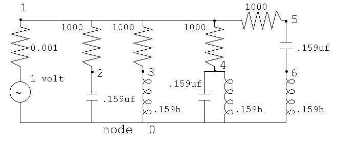 ac_plot.java simple Java plot added
ac_plot.dat capacitor, inductor and tuned circuits
ac_plot.java simple Java plot added
ac_plot.dat capacitor, inductor and tuned circuits
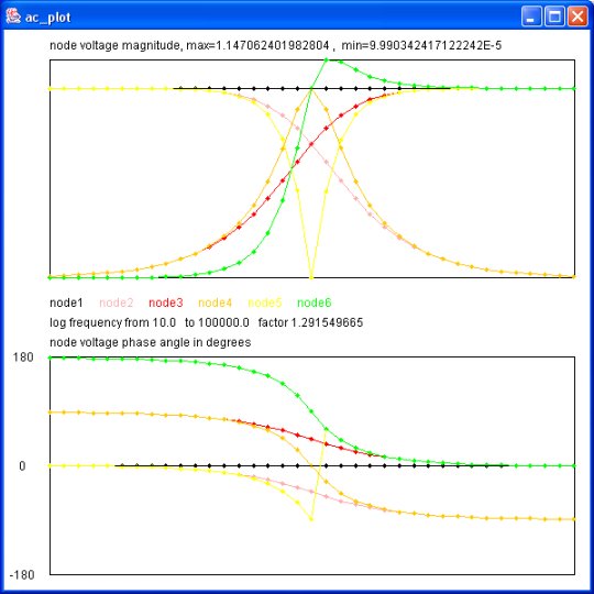 Output of java myjava.ac_plot.java < ac_plot.dat
There are systems of equations with no solutions:
eq1: 1*x + 0*y + 0*z = 2
eq2: 2*x + 0*y + 0*z = 2
eq3: 4*x - 2*y + 3*z = 5
Some may ask: What about solving |A| * |X| = |Y| for X, given A and Y
using |X| = |Y| * |A|^-1 (inverse of matrix A) ?
The reason this is not a good numerical solution is that slightly
more total error will be in the inverse |A|^-1 and then a little
more error will come from the vector times matrix multiplication.
Output of java myjava.ac_plot.java < ac_plot.dat
There are systems of equations with no solutions:
eq1: 1*x + 0*y + 0*z = 2
eq2: 2*x + 0*y + 0*z = 2
eq3: 4*x - 2*y + 3*z = 5
Some may ask: What about solving |A| * |X| = |Y| for X, given A and Y
using |X| = |Y| * |A|^-1 (inverse of matrix A) ?
The reason this is not a good numerical solution is that slightly
more total error will be in the inverse |A|^-1 and then a little
more error will come from the vector times matrix multiplication.
Matrix Inverse
The code for matrix inverse is very similar to the code for solving
simultaneous equations. Added effort is needed to find the
maximum pivot element and there must be both row and column
interchanges. An example that shows the increasing error with the
increasing size of the matrix, on a difficult matrix, is shown below.
Note that results of a 16 by 16 matrix using 64-bit IEEE Floating
point arithmetic that is ill conditioned may become useless.
inverse.f90
test_inverse.f90
test_inverse_f90.out
Extracted form test_inverse_f90.out is
initializing big matrix, n= 2 , n*n= 4
sum of error= 1.84748050191530E-16 , avg error= 4.61870125478825E-17
initializing big matrix, n= 4 , n*n= 16
sum of error= 2.19971263426544E-12 , avg error= 1.37482039641590E-13
initializing big matrix, n= 8 , n*n= 64
sum of error= 0.00000604139304982709 , avg error= 9.43967664035483E-8
initializing big matrix, n= 16 , n*n= 256
sum of error= 83.9630735209012 , avg error= 0.327980755941020
initializing big matrix, n= 32 , n*n= 1024
sum of error= 4079.56590417946 , avg error= 3.98395107830025
initializing big matrix, n= 64 , n*n= 4096
sum of error= 53735.8765782488 , avg error= 13.1191104927365
initializing big matrix, n= 128 , n*n= 16384
sum of error= 85784.2643647822 , avg error= 5.23585597929579
initializing big matrix, n= 256 , n*n= 65536
sum of error= 1097119.16168229 , avg error= 16.7407098645368
initializing big matrix, n= 512 , n*n= 262144
sum of error= 1.36281435213093E+7 , avg error= 51.9872418262837
initializing big matrix, n= 1024 , n*n= 1048576
sum of error= 1.24247404738082E+9 , avg error= 1184.91558778841
Very similar results from the C version:
inverse.c
test_inverse.c
test_inverse.out
inverse.py
test_inverse.py
test_inverse_py.out
test_inv.py numpy version
test_inv_py.out
Extracted form test_inverse.out is
initializing big matrix, n=1024, n*n=1048576
sum of error=1.24247e+09, avg error=1184.92
Inverse.rb Ruby class Inverse
test_inverse.rb Ruby test
test_inverse_rb.out Ruby output
Multiple Precision
A case study using 32-bit IEEE floating point and 50, 100, and 200
digit multiple precision are shown in Lecture 3a
Reducing the number of equation when some values are known
Later, when we study partial differential equations, we will need
cs455_l3c.shtml a process for reducing the number
of equations when we know the value of one or more elements
of the unknown vector.
Nonlinear equations and systems of nonlinear equations
are covered in Lecture 16
Really difficult, are systems of nonlinear equations that need
a solution. The following examples have many comments describing
one or more possible methods of solution:
(Later versions have fewer bugs)
simeq_newton.adb with debug printout
simeq_newton_ada.out
simeq_newton2.adb
simeq_newton2_ada.out
simeq_newton5.adb
test_simeq_newton5.adb
test_simeq_newton5_ada.out
real_arrays.ads used by above
real_arrays.adb used by above
inverse.adb used by above
equation_nl.adb with debug printout
equation_nl_ada.out
simeq_newton.f90 with debug printout
simeq_newton_f90.out
simeq_newton2.f90
simeq_newton2_f90.out
inverse.f90 used by above
udrnrt.f90 used by above
equation_nl.f90 with debug printout
equation_nl_f90.out
simeq_newton.c with debug printout
simeq_newton.out
simeq_newton2.c
simeq_newton2.out
simeq_newton3.h
simeq_newton3.c
test_simeq_newton3.c
test_simeq_newton3_c.out
simeq_newton4.h
simeq_newton4.c
test_simeq_newton4.c
test_simeq_newton4_c.out
invert.h used by above
invert.c used by above
udrnrt.h used by above
udrnrt.c used by above
equation_nl.c with debug printout
equation_nl_c.out
simeq_newton.java with debug printout
simeq_newton2.java
test_simeq_newton2.java
test_simeq_newton2_java.out
simeq_newton3.java
test_simeq_newton3.java
test_simeq_newton3.java
simeq_newton5.java
test_simeq_newton5.java
test_simeq_newton5.java
test_pde_nl.java
test_pde_nl_java.out
test_46_nl.java simple demo
test_46_nl_java.out simple demo
simeq_newton5.py3
test_pde_nl.py3 simple test
test_pde_nl_py3.out simple test
simeq_newton5.java
test_simeq_newton5.java
test_simeq_newton5_java.out
invert.java used by above
equation_nl.java with debug printout
equation_nl_java.out
inverse.java used by above
Accuracy does degrade as the relative size of solution and
matrix elements gets large. Expect similar results with any method.
This program tests 0, 1, 2, 5, ... 1E9, 2E9, 5E9, 1E10 for various n.
simeq_accuracy.c big range test
simeq_accuracy_c.out big range results
Accuracy of all methods degrades with size of matrix on random data.
Not much error for 1024 by 1024 matrix.
Errors increase at 2048 by 2048 and 4096 by 4096.
Over 10K by 10K starts to need multiple precision floating point,
see next lectures.
For your information, modern manufacturing of automobiles:
www.youtube.com/embed/8_lfxPI5ObM?rel=0
The code for matrix inverse is very similar to the code for solving
simultaneous equations. Added effort is needed to find the
maximum pivot element and there must be both row and column
interchanges. An example that shows the increasing error with the
increasing size of the matrix, on a difficult matrix, is shown below.
Note that results of a 16 by 16 matrix using 64-bit IEEE Floating
point arithmetic that is ill conditioned may become useless.


Given a matrix A, computing the inverse AI, then checking that
 |A| * |AI| = |II|  is approximately the identity matrix |I|
is useful and possibly very important.

The check used for this case study was to sum the absolute values
of  |II| - |I| and print the sum and also print the sum divided
by  n*n,  the number of elements in the matrix.

This case study uses the classic, difficult to invert,
variation of the Hilbert Matrix, in floating point format,
shown here as rational numbers:

  | 1/2  1/3  1/4  1/5 |   using i for the column index and
  | 1/3  1/4  1/5  1/6 |   j for the row index,
  | 1/4  1/5  1/6  1/7 |   the (i,j) element is  1/(i+j)
  | 1/5  1/6  1/7  1/8 |   as a floating point number

A few solutions are (A followed by AI):

| 1/2 |  n=1      | 2 |

| 1/2 1/3 |  n=2      |  18  -24 |
| 1/3 1/4 |           | -24   36 |

| 1/2 1/3 1/4 1/5 | n=4   |   200  -1200   2100  -1120 |
| 1/3 1/4 1/5 1/6 |       | -1200   8100 -15120   8400 |
| 1/4 1/5 1/6 1/7 |       |  2100 -15120  29400 -16800 |
| 1/5 1/6 1/7 1/8 |       | -1120   8400 -16800   9800 |

| 1/2  1/3  1/4  1/5  1/6  1/7  1/8  1/9  |
| 1/3  1/4  1/5  1/6  1/7  1/8  1/9  1/10 |
| 1/4  1/5  1/6  1/7  1/8  1/9  1/10 1/11 |
| 1/5  1/6  1/7  1/8  1/9  1/10 1/11 1/12 |
| 1/6  1/7  1/8  1/9  1/10 1/11 1/12 1/13 |
| 1/7  1/8  1/9  1/10 1/11 1/12 1/13 1/14 |
| 1/8  1/9  1/10 1/11 1/12 1/13 1/14 1/15 |
| 1/9  1/10 1/11 1/12 1/13 1/14 1/15 1/16 |

|     2592     -60480      498960    -1995840      4324320     -5189184      3243240     -823680 |
|   -60480    1587600   -13970880    58212000   -129729600    158918760   -100900800    25945920 |
|   498960  -13970880   128066400  -548856000   1248647400  -1553872320    998917920  -259459200 |
| -1995840   58212000  -548856000  2401245000  -5549544000   6992425440   -454053600   118918800 |
|  4324320  -12972960  1248647400  5549544000  12985932960 -16527551040  10821610800 -2854051200 |
| -5189184  158918760 -1553872320  6992425440 -16527551040  21210357168 -13984850880  3710266560 |
|  3243240 -100900800   998917920 -4540536000  10821610800 -13984850880   9275666400 -2473511040 |
|  -823679   25945920  -259459200  1189188000  -2854051200   3710266560  -2473511040   662547600 |

Note the exponential growth of the size of numbers in the inverse.

Now see increasing errors with size of simultaneous equations:
simeq2.c
simeq2.h
simeq2p.h
test_simeq_hilbert.c
test_simeq_hilbert_c.out
Much better accuracy with random matrices
test_simeq_random.c
test_simeq_random_c.out

One measure of the difficulty of inverting a matrix is the size
of the largest diagonal during each step of the inversion process.
The magnitude of the largest element of the inverse will be
approximately the order of the reciprocal of the smallest
of the largest diagonal.

The smallest of the largest diagonal for a few cases are:

n =   2  .277E-1
n =   4  .340E-4
n =   8  .770E-10
n =  16  .560E-22
n =  32  .358E-46
n =  64  .645E-95
n = 128  .178E-192
n = 256  failed with 200 digit multiple precision

The average error, as computed for various precisions, is

        7-digit   15-digit   166-bit    332-bit    664-bit     MatLab
        IEEE      IEEE       mpf        mpf        mpf         IEEE
   n    32-bit    64-bit     50-digit   100-digit  200-digit   64-bit

   2    1.29E-7   4.61E-17   1.99E-59   1.36E-107  6.37E-204   0.00
   4    7.84E-5   1.37E-13   1.91E-58   3.05E-106  6.12E-203   2.39E-13
   8    3.83E0    9.43E-8    4.44E-50   1.81E-98   3.24E-194   7.31E-7
  16    1.23E1    3.27E-1    8.13E-39   2.77E-87   8.56E-183   2.37E2
  32    5.20E0    3.98E0     4.72E-14   4.45E-62   1.19E-158   1.46E6
  64    6.13E0    1.31E1     1.01E8     2.20E-13   1.20E-109   2.55E8
 128    8.39E0    5.23E0     7.79E7     3.46E8     3.83E-12    2.27E10
 256    1.14E3    1.67E1     1.76E8     8.51E7     1.05E8      8.38E11

The errors bigger than E-5 are very deceiving
in the first two columns. They indicate failure to invert.
MatLab does indicate failure for n=16 and larger, other codes had
the matrix singular error suppressed.

A reasonable conclusion, for this matrix, is that an n by n matrix
needs more than n bits of floating point precision in order to
get a reliable inverse. Twice the number of bits as n to get
good results.

Before you panic, notice the results for the same test in MatLab
for this hard to invert matrix verses a pseudo random matrix.

n=2,   avgerr=0            , rnderr=4.16334e-017
n=4,   avgerr=2.39808e-013 , rnderr=1.04246e-016
n=8,   avgerr=7.31534e-007 , rnderr=7.86263e-016
n=16,  avgerr=237.479      , rnderr=3.57e-016
n=32,  avgerr=1.46377e+006 , rnderr=7.5899e-016
n=64,  avgerr=2.55034e+008 , rnderr=2.34115e-015
n=128, avgerr=2.2773e+010  , rnderr=6.70795e-015
n=256, avgerr=8.38903e+011 , rnderr=1.9137e-014

Well conditioned matrices may be inverted for n in the range
10,000 to 20,000 with IEEE 64-bit floating point.
Many large matrices are sparse, having many zero elements,
and may have only bands of non zero elements. Unfortunately
the inverse of sparse matrices are not sparse, thus
sparse matrix storage techniques may actually be slower.

The MatLab code is, of course, the shortest (stripped here):
  n=1;
  for r=1:8
    n=2*n;
    A=zeros(n,n);
    B=rand(n,n);
    for i=1:n
      for j=1:n
        A(i,j)=1.0/(i+j);
      end
    end
    avgerr=sum(sum(abs(A*inv(A)-eye(n,n))))/(n*n)
    rnderr=sum(sum(abs(B*inv(B)-eye(n,n))))/(n*n)
  end

The detailed code and results are:

invrnd.m actual MatLab code
invrnd_m.out file output
invrnd_mm.out partial screen output

inverse.f90 basic inverse
test_inverse.f90 test program
test_inverse_f90.out output

inverse.py basic inverse
test_inverse.fpy test program
test_inverse_py.out output

Simeq.scala has inverse
TestSimeq.scala test has inverse
TestSimeq_scala.out output has inverse

Extracted form test_inverse_f90.out is
initializing big matrix, n= 2 , n*n= 4
 sum of error= 1.84748050191530E-16 , avg error= 4.61870125478825E-17
initializing big matrix, n= 4 , n*n= 16
 sum of error= 2.19971263426544E-12 , avg error= 1.37482039641590E-13
initializing big matrix, n= 8 , n*n= 64
 sum of error= 0.00000604139304982709 , avg error= 9.43967664035483E-8
initializing big matrix, n= 16 , n*n= 256
 sum of error= 83.9630735209012 , avg error= 0.327980755941020
initializing big matrix, n= 32 , n*n= 1024
 sum of error= 4079.56590417946 , avg error= 3.98395107830025
initializing big matrix, n= 64 , n*n= 4096
 sum of error= 53735.8765782488 , avg error= 13.1191104927365
initializing big matrix, n= 128 , n*n= 16384
 sum of error= 85784.2643647822 , avg error= 5.23585597929579
initializing big matrix, n= 256 , n*n= 65536
 sum of error= 1097119.16168229 , avg error= 16.7407098645368
initializing big matrix, n= 512 , n*n= 262144
 sum of error= 1.36281435213093E+7 , avg error= 51.9872418262837
initializing big matrix, n= 1024 , n*n= 1048576
 sum of error= 1.24247404738082E+9 , avg error= 1184.91558778841


Very similar results from the C version:

inverse.c
inverse.h
test_inverse.c
test_inverse.out

Similar results from float rather than double in the C version:

inversef.c
inversef.h
test_inversef.c
test_inversef.out


Exploring results from 50 digit multiple precision arithmetic version:

mpf_inverse.c
mpf_inverse.h
test_mpf_inverse.c
test_mpf50_inverse.out

Changing 'digits' to 100 digit multiple precision arithmetic version:

test_mpf100_inverse.out

Changing 'digits' to 200 digit multiple precision arithmetic version:

test_mpf200_inverse.out

The 200 digit run with more output:

test_mpf_inverse.out

Java version, double

inverse.java
test_inverse.java
test_inverse_java.out

Java version, BigDecimal 300 bits or more

Big_inverse.java
test_Big_inverse.java
test_Big_inverse_java.out

Big_simeq.java
test_Big_simeq.java
test_Big_simeq_java.out
time_Big_simeq.java
time_Big_simeq_java.out

Big_nuderiv.java
test_Big_nuderiv
test_Big_nuderiv_java.out

Ada version, double

hilbert_inverse.adb
hilbert_inverse_ada.out

Ada version 50, 100 and 200 digits

digits_hilbert_inverse.adb
digits_hilbert_inverse_ada_50.out
digits_hilbert_inverse_ada_100.out
digits_hilbert_inverse_ada_200.out

Basic gcc stack storage limitation prevented getting all output.
Even happens on 64-bit computer with 8GB or RAM.
We have a number of clusters at UMBC, I happen to have used
our Bluegrit, Bluewave, Tara and Maya and Taki clusters and the
MPI examples are from these multi processor machines.
For multi core machines, there are Java Threads and
"C" pthreads and Ada tasks. I have a 12 core desktop
and Intel has a many core computer.
Examples are presented below.
At the end are a few multi core benchmarks for you to run.
We can use our biggest super computer on campus, Taki.

NOTE:
MPI is running on a distributed memory system.
Each process may be considered to have local memory and
in general, there is no common shared memory.

Multicore machines are described here as shared memory systems.
All memory is available to all threads and tasks.
Also know technically as a single address space.

Some parallel programming techniques apply to both
distributes and shared memory, some techniques do not
apply to both memory systems.


MPI
MPI stands for Message Passing Interface and is
available on many multiprocessors. MPI may be installed
as the open source version MPICH. There are other
software libraries and languages for multiprocessors,
yet, this lecture only covers MPI.

The WEB page here at UMBC is
www.csee.umbc.edu/help/MPI

Programming in MPI is the SPMD Single Program Multiple Data style of
programming. One program runs on all CPU's in the multiprocessor.
Each CPU has a number, called a rank in MPI, called myid in my code and
called node or node number in comments.

"if-then-else" code may be based on node number is used to have
unique computation on specific nodes. There is a master node,
typically the node with rank zero in MPI. The node number may
also be used in index expressions and other computation. Many
MPI programs use the master as a number cruncher along with the
other nodes in addition to the master serving as overall control
and synchronization.

Examples below are given first in "C" and then a few in Fortran.
Other languages may interface with the MPI library.
These just show a simple MPI use, these are combined later for
solving simultaneous equations on a multiprocessor.

Just check that a message can be sent and received from each
node, processor, CPU, etc. numbered as "rank".

roll_call.c

roll_call.out

Just scatter unique data from the "master" to all nodes.
Then gather the unique results from all nodes.

scat.c

scat.out

Here is the Makefile I used.
Makefile for C on Bluegrit cluster


Repeating the "roll_call" just changing the language to Fortran.

roll_call.F

roll_call_F.out

Repeating scatter/gather just changing the language to Fortran.

scat.F

scat_F.out

The Fortran version of the Makefile with additional files I used.

Makefile for Fortran on Bluegrit cluster

my_mpif.h only needed if not on cluster

nodes only needed if default machinefile not used

MPI Simultaneous Equations

Now, the purpose of this lecture, solve huge simultaneous
equations on a highly parallel multiprocessor.

Well, start small when programming a multiprocessor and print out
every step to be sure the indexing and communication is exactly
correct.

This is hard to read, yet it was a necessary step.

psimeq_debug.c

psimeq_debug.out

Then, some clean up and removing or commenting out most debug print:

psimeq1.c

psimeq1.out

The input data was created so that the exact answers were 1, 2, 3 ...
It is interesting to note: because the data in double precision floating
point was from the set of integers, the answers are exact for
8192 equations in 8192 unknowns.

psimeq1.out8192

|A| * |X| = |Y|  given matrix |A| and vector |Y| find vector |X|

  | 1 2 3 4 5 | |5| | 35|  for 5 equations in 5 unknowns
  | 2 2 3 4 5 | |4| | 40|  the solved problem is this
  | 3 3 3 4 5 |*|3|=| 49|
  | 4 4 4 4 5 | |2| | 61|
  | 5 5 5 5 5 | |1| | 75|

A series of timing runs were made, changing the number of equations.
The results were expected to increase in time as order n^3 over the
number of processors being used. Reasonable agreement was measured.

Using 16 processors:
Number of  Time computing  Cube root of
equations  solution (sec)  16 times Time (should approximately double
    1024       3.7          3.9           as number of equations double)
    2048      17.2          6.5
    4096      83.5         11.0
    8192     471.9         19.6

More work may be performed to minimize the amount of
data send and received in "rbuf".


C pthreads Simultaneous Equations
Basic primitive barrier in C pthreads
run_thread.c
run_thread_c.out

Simultaneous equation solution using AMD 12 core
tsimeq.h
tsimeq.c
time_tsimeqb.c
time_tsimeqb.out

More examples of pthreads with debug printout
thread_loop.c with comments
thread_loop_c.out


Java Simultaneous Equations

Java threads are demonstrated by the following example.
RunThread.java
When run, there are four windows, each showing a dot as that thread runs.
RunThread.out
Note that CPU and Wall time are measured and printed. (on some Java versions)

The basic structure of threads needed for my code:
(I still have not figured out why I need the dumb "sleep" in 2)
Barrier2.java
Barrier2_java.out
(OK, several versions later)
CyclicBarrier4.java
CyclicBarrier4_java.out

Simultaneous equation solution with multiple processors in
a shared memory configuration is accomplished with:

psimeq.java
test_psimeq.java test driver
test_psimeq_java.out output
psimeq_dbg.java with lots of debug print
test_simeq_dbg.java with debug
test_psimeq_dbg_java.out output with debug
A better version making better use of threads and cyclic barrier:
simeq_thread.java
test_simeq_thread.java test driver
test_simeq_thread_java.out output

And, test results for "diff" the non threaded version
test_simeq_java.out output

Some crude timing tests:
time_simeq.java test driver
time_pimeq_java.out output
time_psimeq.java test driver
time_psimeq_java.out output yuk!
time_simeq_thread.java test driver
time_pimeq_thread_java.out output quad core


Ada Simultaneous Equations

Simultaneous equation solution with multiple processors in
a shared memory configuration is accomplished with:

psimeq.adb
test_psimeq.adb test driver
test_psimeq_ada.out output
psimeq_dbg.adb with lots of debug print
test_simeq_dbg.adb with debug
test_psimeq_dbg_ada.out output with debug
time_psimeq.adb test driver
time_psimeq_ada.out outputs

Then using Barriers
bsimeq_2.adb
time_bsimeq.adb test driver
time_bsimeq_ada.out outputs

Another tutorial type example
task_loop.adb with comments
task_loop_ada.out


Python Simultaneous Equations

The basic structure of threads needed for my code (python2):
barrier2.py
barrier2_py.out


Multiprocessor Benchmarks

"C" pthreads are demonstrated by an example that measures the
efficiency of two cores, four cores or eight cores.
time_mp2.c
time_mp2.out

The ratio of Wall time to CPU time indicates degree of parallelism.

time_mp4.c 4 core shared memory
time_mp4.out

time_mp8.c 8 core shared memory
time_mp8_c.out

My AMD 12-core desktop computer July 2010
time_mp12.c 12 core shared memory
time_mp12_c.out

time_mp4.java 4 core shared memory
time_mp4_java.out

time_mp8.java 8 core shared memory
time_mp8_java.out


pthreads using mutex.c and mutex.h
mutex.c encapsulate pthreads
mutex. encapsulate pthreads
thread4m.c main plus 4 threads
thread4m_c.out output
thread11m.c main plus 11 threads
thread11m_c.out output

for comparison, using just basic pthreads
thread4.c main plus 4 threads
thread4_c.out output

Comparison using Java threads, C pthreads  on big  matrix multiply
 c[1000][1000] = a[1000][1000] * b[1000][1000]
 for comparison, one thread time and four thread time:
Java example
matmul_thread4.java source code
matmul_thread4_java.out output
matmul_thread1.java source code no threads
matmul_thread1_java.out output

C pthread example
matmul_pthread4.c source code
matmul_pthread4.out output
matmul.c source code no threads
matmul_c.out output

Python3 threading and multitasking
thread3.py3 source code
thread3_py3.out output
multi.py3 source code
multi_py3.out output

C OpenMP example  1000 caused segfault, cut to 510
omp_matmul.c source code
omp_matmul.out output
Given numeric data points, find an equation that approximates the data
with a least square fit. This is one of many techniques for getting
an analytical approximation to numeric data.
The problem is stated as follows :
Given measured data for values of Y based on values of X1,X2 and X3. e.g.
Y_actual X1 X2 X3 observation, i
-------- ----- ----- -----
32.5 1.0 2.5 3.7 1
7.2 2.0 2.5 3.6 2
6.9 3.0 2.7 3.5 3
22.4 2.2 2.1 3.1 4
10.4 1.5 2.0 2.6 5
11.3 1.6 2.0 3.1 6
Find a, b and c such that Y_approximate = a * X1 + b * X2 + c * X3
and such that the sum of (Y_actual - Y_approximate) squared is minimized.
(We are minimizing RMS error.)
The method for determining the coefficients a, b and c follows directly
form the problem definition and mathematical analysis given below.
Set up and solve the system of linear equations:
(Each SUM is for i=1 thru 6 per table above, note symmetry)
| SUM(X1*X1) SUM(X1*X2) SUM(X1*X3) | | a | | SUM(X1*Y) |
| SUM(X2*X1) SUM(X2*X2) SUM(X2*X3) | x | b | = | SUM(X2*Y) |
| SUM(X3*X1) SUM(X3*X2) SUM(X3*X3) | | c | | SUM(X3*Y) |
Easy to program, not good data:
lsfit_lect.c
lsfit_lect_c.out
lsfit_lect.java
lsfit_lect_java.out
lsfit_lect.py
lsfit_lect_py.out
lsfit_lect.f90
lsfit_lect_f90.out
lsfit_lect.m similar to c
lsfit_lect_m.out
test_lsfit.py3 Python3 two methods
test_lsfit_py3.out output
test_lsfit2.py3 Python3 two methods
test_lsfit2_py3.out output better
Now, suppose you wanted a constant term to make the fit:
Y_approximate = Y0 + a * X1 + b * X2 + c * X3
Then the linear equations would be:
| SUM( 1* 1) SUM( 1*X1) SUM( 1*X2) SUM( 1*X3) | | Y0 | | SUM( 1*Y) |
| SUM(X1* 1) SUM(X1*X1) SUM(X1*X2) SUM(X1*X3) | | a | | SUM(X1*Y) |
| SUM(X2* 1) SUM(X2*X1) SUM(X2*X2) SUM(X2*X3) | x | b | = | SUM(X2*Y) |
| SUM(X3* 1) SUM(X3*X1) SUM(X3*X2) SUM(X3*X3) | | c | | SUM(X3*Y) |
Note the symmetry! Easy to program.
Note the simultaneous equations, from Lecture 3: |A| x |X| = |Y|
|A| and |Y| easily computable, solve for |X| to get Y0, a, b and c
We now have a simple equation to compute Y approximately from a reasonable
range of X1, X2, and X3.
Y is called the dependent variable and X1 .. Xn the independent variables.
The procedures below implement a few special cases and the general case.
The number of independent variables can vary, e.g. 2D, 3D, etc. .
The approximation equation may use powers of the independent variables
The user may create additional independent variables e.g. X2 = SIN(X1)
with the restriction that the independent variables are linearly
independent. e.g. Xi not equal p Xj + q for all i,j,p,q
Mathematical derivation
The mathematical derivation of the least square fit is as follows :
Given data for the independent variable Y in terms of the dependent
variables S,T,U and V consider that there exists a function F
such that Y = F(S,T,U,V)
The problem is to find coefficients a,b,c and d such that
Y_approximate = a * S + b * T + c * U + d * V
and such that the sum of ( Y - Y_approximate ) squared is minimized.
Note: a, b, c, d are scalars. S, T, U, V, Y, Y_approximate are vectors.
To find the minimum of SUM((Y - Y_approximate)^2)
the derivatives must be taken with respect to a,b,c and d and
all must equal zero simultaneously. The steps follow :
SUM((Y - Y_approximate)^2) = SUM((Y - a*S - b*T - c*U - d*V)^2)
d/da = -2 * S * SUM( Y - a*S - b*T - c*U - d*V )
d/db = -2 * T * SUM( Y - a*S - b*T - c*U - d*V )
d/dc = -2 * U * SUM( Y - a*S - b*T - c*U - d*V )
d/dd = -2 * V * SUM( Y - a*S - b*T - c*U - d*V )
Setting each of the above equal to zero (derivative minimum at zero)
and putting constant term on left, the -2 is factored out,
the independent variable is moved inside the summation
SUM( a*S*S + b*S*T + c*S*U + d*S*V = S*Y )
SUM( a*T*S + b*T*T + c*T*U + d*T*V = T*Y )
SUM( a*U*S + b*U*T + c*U*U + d*U*V = U*Y )
SUM( a*V*S + b*V*T + c*V*U + d*V*V = V*Y )
Distributing the SUM inside yields
a * SUM(S*S) + b * SUM(S*T) + c * SUM(S*U) + d * SUM(S*V) = SUM(S*Y)
a * SUM(T*S) + b * SUM(T*T) + c * SUM(T*U) + d * SUM(T*V) = SUM(T*Y)
a * SUM(U*S) + b * SUM(U*T) + c * SUM(U*U) + d * SUM(U*V) = SUM(U*Y)
a * SUM(V*S) + b * SUM(V*T) + c * SUM(V*U) + d * SUM(V*V) = SUM(V*Y)
To find the coefficients a,b,c and d solve the linear system of equations
| SUM(S*S) SUM(S*T) SUM(S*U) SUM(S*V) | | a | | SUM(S*Y) |
| SUM(T*S) SUM(T*T) SUM(T*U) SUM(T*V) | x | b | = | SUM(T*Y) |
| SUM(U*S) SUM(U*T) SUM(U*U) SUM(U*V) | | c | | SUM(U*Y) |
| SUM(V*S) SUM(V*T) SUM(V*U) SUM(V*V) | | d | | SUM(V*Y) |
Some observations :
S,T,U and V must be linearly independent.
There must be more data sets (Y, S, T, U, V) than variables.
The analysis did not depend on the number of independent variables
A polynomial fit results from the substitutions S=1, T=x, U=x^2, V=x^3
The general case for any order polynomial of any number of variables
may be used with a substitution, for example, S=1, T=x, U=y, V=x^2,
W=x*y, X= y^2, etc to terms such as exp(x), log(x), sin(x), cos(x).
Any number of terms may be used. The "1" is for the constant term.
Using the S,T,U,V notation above, fitting Y_approx to find a, b, c, d
Y_approx = a*S + b*T + c*U + d*V + ...
Choose S = 1.0 thus a is the constant term
Choose T = log(x) thus b is the coefficient of log(x)
Choose U = log(x*x) thus c is the coefficient of log(x*x)
Choose V = sin(x) thus d is the coefficient of sin(x)
see 4 additional terms in lsfit_log.c
Thus our x data, n = 21 samples in code, is fit to
Y_approx = a + b*log(x) + c*log(x*x) + d*sin(x) + ...
By putting the terms in a vector, simple indexing builds the matrix:
A[i][j] = A[i][j] + term_i * term_j summing over n terms using k
lsfit_log.c fitting log and other terms
lsfit_log_c.out
fitting a simple polynomial, 1D
Now, suppose you wanted to fit a simple polynomial:
Given the value of Y for at least four values of X,
Y_approximate = C0 + C1 * X + C2 * X^2 + C3 * X^3
Then the linear equations would be A*X=Y:
| SUM(1 *1) SUM(1 *X) SUM(1 *X^2) SUM(1 *X^3) | | C0 | | SUM(1 *Y) |
| SUM(X *1) SUM(X *X) SUM(X *X^2) SUM(X *X^3) | | C1 | | SUM(X *Y) |
| SUM(X^2*1) SUM(X^2*X) SUM(X^2*X^2) SUM(X^2*X^3) |x| C2 | = | SUM(X^2*Y) |
| SUM(X^3*1) SUM(X^3*X) SUM(X^3*X^2) SUM(X^3*X^3) | | C3 | | SUM(X^3*Y) |
Note that the (i,j) subscript in the A matrix has SUM(X^(i)*X^(j))
for i=0..3, j=0..3
In C, to build A matrix and Y vector for solving simultaneous equations:
// sample polynomial least square fit, nth power, m values of xd and yd
for(i=0; i<n+1; i++)
{
for(j=0; j<n+1; j++)
{
A[i][j] = 0.0;
}
Y[i] = 0.0;
}
for(k=0; k<m; k++)
{
y = yd[k];
x = xd[k];
pwr[0] = 1.0;
for(i=1; i<=n+1; i++) pwr[i] = pwr[i-1]*x;
for(i=0; i<n+1; i++)
{
for(j=0; j<n+1; j++)
{
A[i][j] = A[i][j] + pwr[i]*pwr[j]; // SUM
}
Y[i] = Y[i] + y*pwr[i];
}
}
Solve the simultaneous equations A*X=Y for X[0]=C0, X[1]=C1, X[2]=C2, X[3]=C3
Note that the sum is taken over all observations and the "1" is
just shown to emphasize the symmetry.
Sample code in various languages:
least_square_fit.c really old
least_square_fit_c.out
least_square.py3
least_square_py3.out
test_lsfit.py3 Python3 two methods
test_lsfit_py3.out output
lsfit.py3 just 1D version for copying
peval.py3 just 1D version for copying
least_square_fit.f90
least_square_fit_f90.out
Least_square.rb Ruby class new
test_least_square.rb test
test_least_square_rb.out test output
least_square_fit.java
least_square_fit_java.out
least_square_fit_3d.java
least_square_fit_3d_java.out
least_square_fit_4d.java
least_square_fit_4d_java.out
A specialized version for use later with PDE's
lsfit.java
test_lsfit.java
test_lsfit_java.out
test_lsfit2.java
test_lsfit2_java.out
test_lsfit3.java
test_lsfit3_java.out
test_lsfit4.java
test_lsfit4_java.out
test_lsfit5.java
test_lsfit5_java.out
test_lsfit6.java
test_lsfit6_java.out
test_lsfit7.java
test_lsfit7_java.out
uses simeq.java
The Makefile entry that makes test_lsfit_java.out
test_lsfit_java.out: test_lsfit.java lsfit.java simeq.java
javac -cp . simeq.java
javac -cp . lsfit.java
javac -cp . test_lsfit.java
java -cp . test_lsfit > test_lsfit_java.out
rm -f *.class
least_square_fit.adb
least_square_fit_ada.out
least_square_fit_2d.adb
least_square_fit_2d_ada.out
least_square_fit_3d.adb
least_square_fit_3d_ada.out
least_square_fit_4d.adb
least_square_fit_4d_ada.out
real_arrays.ads
real_arrays.adb
lsfit.ads has 1D through 6D
lsfit.adb
test_lsfit6.adb
test_lsfit6_ada.out
array4d.ads
test_lsfit5.adb
test_lsfit5_ada.out
array5d.ads
test_lsfit4.adb
test_lsfit4_ada.out
array4d.ads
test_lsfit3.adb
test_lsfit3_ada.out
array3d.ads
test_lsfit2.adb
test_lsfit2_ada.out
integer_arrays.ads
integer_arrays.adb
real_arrays.ads
real_arrays.adb
The Makefile entry to make test_lsfit6_ada.out
test_lsfit6_ada.out: test_lsfit6.adb lsfit.ads lsfit.adb \
array3d.ads array4d.ads array5d.ads array6d.ads \
real_arrays.ads real_arrays.adb \
integer_arrays.ads integer_arrays.adb
gnatmake test_lsfit6.adb
./test_lsfit6 > test_lsfit6_ada.out
rm -f test_lsfit
rm -f *.ali
rm -f *.o
similarly for test_lsfit2_ada.out, test_lsfit3_ada.out,
test_lsfit4_ada.out, test_lsfit5_ada.out
Similar code in plain C (up to 7th power in up to 6 or 4 dimensions)
lsfit.h
lsfit.c
test_lsfit.c
test_lsfit_c.out
test_lsfit7.c
test_lsfit7_c.out
test_write_lsfit7.c
test_write_lsfit7_c.out
test_write_lsfit71.c generated
test_write_lsfit72.c generated
Simple one variable versions polyfit polyval
polyfit.h
polyfit.c
polyval.h
polyval.c
test_polyfit.c
test_polyfit_c.out
test_polyfit.py3
test_polyfit_py3.out
test_polyfit_py3.png
poly.java
test_poly.java
test_poly_java.out
Poly.scala
Test_poly.scala
Test_poly_scala.out
truncated series vs lsfit for sin(x+y) and sin(x+y+z)
using code from above, another test case:
fit_sin.adb demonstrates that a lsfit to a specified power,
does not give the same coefficients as a truncated approximation,
to the same power, and is a more accurate fit.
fit_sin.adb
fit_sin_ada.out
comparison to very small Matlab code
generic_real_least_square_fit.ada
lsfit.m MatLab source code (tiny!)
lsfit_m.out MatLab output and plot

comparison to small Python code
test_polyfit.py Python source code
test_polyfit_py.out Python output and plot
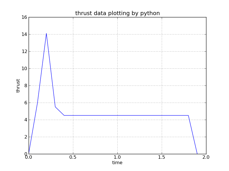
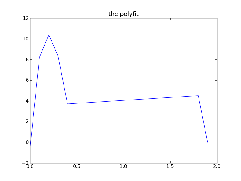


Terms for fitting two and three variables, 2D and 3D
And to see how polynomials in two and three variables may be fit:
Given a value of Y for each value of X, get polynomial with X^2
Y_approximate = C0 + C1 * X + C2 * X^2
Then the linear equations would be:
| SUM(1 *1) SUM(1 *X) SUM(1 *X^2) | | C0 | | SUM(1 *Y) |
| SUM(X *1) SUM(X *X) SUM(X *X^2) | | C1 | | SUM(X *Y) |
| SUM(X^2*1) SUM(X^2*X) SUM(X^2*X^2) |x| C2 | = | SUM(X^2*Y) |
Given a value of Y for each value of X, get polynomial with X^3
Y_approximate = C0 + C1 * X + C2 * X^2 + C3 * X^3
Then the linear equations would be:
| SUM(1 *1) SUM(1 *X) SUM(1 *X^2) SUM(1 *X^3) | | C0 | | SUM(1 *Y) |
| SUM(X *1) SUM(X *X) SUM(X *X^2) SUM(X *X^3) | | C1 | | SUM(X *Y) |
| SUM(X^2*1) SUM(X^2*X) SUM(X^2*X^2) SUM(X^2*X^3) |x| C2 | = | SUM(X^2*Y) |
| SUM(X^3*1) SUM(X^3*X) SUM(X^3*X^2) SUM(X^3*X^3) | | C3 | | SUM(X^3*Y) |
Note that index [i][j] of the matrix has SUM(X^i*X^j)) when subscripts 0..3
Note that the terms for two and three variables in a polynomial are:
two three can optimize
a^0 b^0 a^0 b^0 c^0 constant, "1"
a^1 b^0 a^1 b^0 c^0 just a
a^0 b^1 a^0 b^1 c^0 just b
a^0 b^0 c^1
a^2 b^0 a^2 b^0 c^0 just a^2
a^1 b^1 a^1 b^1 c^0 a*b
a^0 b^2 a^1 b^0 c^1
a^0 b^2 c^0
a^0 b^1 c^1
a^0 b^0 c^2
Then terms with a sum of the powers equal to 3, 4, 5, 6 are available
Note that the matrix has the first row as the sum of each term
multiplied by the first term. The second row is the sum of each
term multiplied by the second term, etc.
The data for the terms is from the raw data sets of
y_actual a b or y_actual a b c
being used to determine a fit
y_approx=F(a,b) or y_approx=F(a,b,c)
Terms for the data point y1 a1 b1 are:
1 a1 b1 a1^2 a1*b1 b1^2 the constant term y1
These terms are multiplied by the first term, "1" and added to row 1.
These terms are multiplied by the second term, "a1" and added to row 2, etc.
Then the terms for data point y2 a2 b2 are:
1 a2 b2 a2^2 a2*b2 b2^2 the constant term y2
These terms are multiplied by the first term, "1" and added to row 1.
These terms are multiplied by the second term, "a2" and added to row 2, etc.
Then the simultaneous equations are solved for the coefficients C1, C2, ...
to get the approximating function
y_approx = F(a,b) = C1 + C2*a + C3*b + C4*a^2 + C5*a*b + C6*b^2
The following sample programs compute the least square fit of
internally generated data for low polynomial powers and compute
the accuracy of the fit in terms of root-mean-square error,
average error and maximum error. Note that the fit becomes exact
when the data is from a low order polynomial and the fit uses at
least that order polynomial.
least_square_fit_2d.c
least_square_fit_2d.out
least_square_fit_3d.c
least_square_fit_3d.out
least_square_fit_4d.c
least_square_fit_4d.out
least_square_fit2d.adb
least_square_fit2d_ada.out
real_arrays.ads
real_arrays.adb
Development of Python 2d and 3d least square fit
polyfit2.py3
polyfit2_py3.out
polyfit3.py3
polyfit3_py3.out
You can translate the above to your favorite language.
Now, if everything works, a live interactive demonstration of
least square fit.
The files needed are:
Matrix.java
LeastSquareFit.java
LeastSquareFitFrame.java
LeastSquareFit.out
LeastSquareFitAbout.txt
LeastSquareFitHelp.txt
LeastSquareFitEvaluate.txt
LeastSquareFitAlgorithm.txt
LeastSquareFitIntegrate.txt
The default parameter is an n, all, point fit.
Then set parameter to 3, for n=3, third order polynomial fit.
Then set parameter to 4 and 5 to see improvement.
Homework 2
Spline fit, possible demonstration
There are many other ways to fit a set of points.
The Spline fit smooths the fit by controlling derivatives.
SplineFrame.java
(Replace "LeastSquareFit" with "Spline" then get same files as above.)
Demonstration to see a different type of fit.
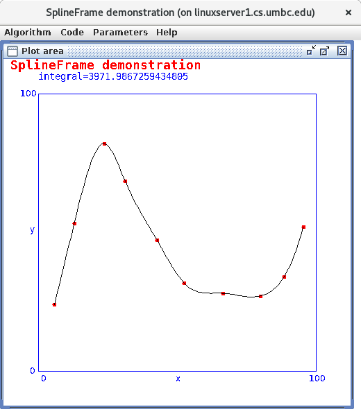 Right click on points, left to right increasing X.
Left click to see plot.
Optional lecture on taylor fit to implement math functions
that may not be availabke in programming language you are using.
optional lecture 4.5
updated 10/30/2021
Right click on points, left to right increasing X.
Left click to see plot.
Optional lecture on taylor fit to implement math functions
that may not be availabke in programming language you are using.
optional lecture 4.5
updated 10/30/2021
A polynomial of degree n has the largest exponent value n.
There are n+1 terms and n+1 coefficients.
A normalized polynomial has the coefficient of the
largest exponent equal to 1.0.
An nth order polynomial with coefficients c_0 through c_n.
y = c_0 + c_1 x + c_2 x^2 +...+ c_n-1 x^n-1 + c_n x^n
Horners method for evaluating a polynomial
"y" is computed numerically using Horners method that
needs n multiplications and n additions.
Thus faster and more accurate.
Starting at the highest power, set y = c_n * x
Then combine the next coefficient y = (c_n-1 + y) * x
Continue for c_n-2 until c_1 y = (c_1 + y) * x
Then finish y = c_0 + y
The code in C, Fortran 90, Java and Ada 95 is:
/* peval.c Horners method for evaluating a polynomial */
double peval(int n, double x, double c[])
{ /* an nth order polynomial has n+1 coefficients */
/* stored in c[0] through c[n] */
/* y = c[0] + c[1]*x + c[2]*x^2 +...+ c[n]*x^n */
int i;
double y = c[n]*x;
if(n<=0) return c[0];
for(i=n-1; i>0; i--) y = (c[i]+y)*x;
return y+c[0];
} /* end peval */
! peval.f90 Horners method for evaluating a polynomial
function peval(n, x, c) result (y)
! an nth order polynomial has n+1 coefficients
! stored in c(0) through c(n)
! y = c(0) + c(1)*x + c(2)*x^2 +...+ c(n)*x^n
implicit none
integer, intent(in) :: n
double precision, intent(in) :: x
double precision, dimension(0:n), intent(in) :: c
double precision :: y
integer i
if(n<=0) y=c(0); return
y = c(n)*x
do i=n-1, 1, -1
y = (c(i)+y)*x
end do
y = y+c(0)
end function peval
// peval.java Horners method for evaluating a polynomial
double peval(int n, double x, double c[])
{ // an nth order polynomial has n+1 coefficients
// stored in c[0] through c[n]
// y = c[0] + c[1]*x + c[2]*x^2 +...+ c[n]*x^n
double y = c[n]*x;
if(n<=0) return c[0];
for(int i=n-1; i>0; i--) y = (c[i]+y)*x;
return y+c[0];
} // end peval
-- peval.adb Horners method for evaluating a polynomial
function peval(n : integer; x : long_float; c : vector) return long_float is
-- an nth order polynomial has n+1 coefficients
-- stored in c(0) through c(n)
-- y := c(0) + c(1)*x + c(2)*x^2 +...+ c(n)*x^n
y : long_float;
begin
if n<=0 then return c(0); end if;
y := c(n)*x;
for i in reverse 1..n-1 loop -- do i:=n-1, 1, -1
y := (c(i)+y)*x;
end loop;
y := y+c(0);
return y;
end peval;
MatLab
y = polyval(c, x)
Python
from numpy import polyval
y = polyval(c, x)
Testing high degree polynomials
Although Horners method is fast and accurate on most polynomials,
the following test programs in C, Fortran 90, Java and Ada95
show that evaluating polynomials of order 9 and 10 can have
significant absolute error.
The test programs generate a set of roots r_0, r_1, ...
and computer the coefficients of a set of polynomials
y = (x-r_0)*(x-r_1)*...*(x-r_n-1) becomes
y = c_0 + c_1*x + c_2*x^2 +...+ c_n-1*x^n-1 + 1.0*x^n
when x is any of the roots, y should be zero.
Study one of the .out files and see how the absolute
error increases with polynomial degree and increases with
the magnitude of the root.
(The source code was run on various types of computers
and various operating systems. Results vary.)
peval.c
peval_c.out
peval.f90
peval_f90.out
peval.java
peval_java.out
peval.adb
peval_ada.out
test_peval.rb
test_peval_rb.out
Having the coefficients of a polynomial allows creating
the derivative and integral of the polynomial.
Derivative of Polynomial
Given:
y = c_0 + c_1 x + c_2 x^2 +...+ c_n-1 x^n-1 + c_n x^n
dy/dx = c_1 + 2 c_2 x + 3 c_3 x^2 +...+ n-1 c_n-1 x^n-2 + n c_n x^n-1
The coefficients of dy/dx may be called cd and computed:
for(i=0; i<n; i++) cd[i] = (double)(i+1)*c[i+1];
nd = n-1;
The derivative may be computed an any point, example x=a, using
dy_dx_at_a = peval(nd, a, cd);
Integral of Polynomial
Similarly, the integral y(x) dx has coefficients
Given:
y = c_0 + c_1 x + c_2 x^2 +...+ c_n-1 x^n-1 + c_n x^n
int_y_dx = 0 + c_0 x + c_1/2 x^2 +...+ c_n-1/n x^n + c_n/(n+1) x^n+1
The coefficients of int_y_dy may be called ci and computed:
ci[0] = 0.0; /* a reasonable choice */
ni = n+1;
for(i=1; i<=ni; i++) ci[i] = c[i-1]/(double)i;
The integral of the original polynomial y from a to b is computed:
int_y_a_b = peval(ni, b, ci) - peval(ni, a, ci);
Polynomial Arithmetic
The sum, difference, product and quotient of two polynomials p and q are:
(unused locations filled with zeros)
nsum = max(np,nq);
for(i=0; i<=nsum; i++) sum[i] = p[i] + q[i];
ndifference = max(np,nq);
for(i=0; i<=ndifference; i++) difference[i] = p[i] - q[i];
nproduct = np+nq;
for(i=0; i<=nproduct; i++) product[i] = 0.0;
for(i=0; i<=np; i++)
for(j=0; j<=nq; j++) product[i+j] += p[i]*q[j];
/* np > nd */
nquotient = np-nd;
nremainder = np
k = np;
for(j=0; j<=np; j++) r[j] = p[j]; /* initial remainder */
for(i=nquotient; i>=0; i--)
{
quotient[i] = r[k]/d[nd]
for(j=nd; j>=0; j--) r[k-nd+j] = r[k-nd+j] - quotient[i]*d[j]
k--;
}
Polynomial operations including add,sub,mul,div,roots,deriv,integral
poly.h
poly.c
test_poly.c
test_poly_c.out
poly.java
test_poly.java
test_poly_java.out
In Python all available import numpy.matlib
To see all functions print dir(numpy.matlib)
Polynomial series
Taylor series, for any differentiable function, f(x)
(x-a) f'(a) (x-a)^2 f''(a) (x-a)^3 f'''(a)
f(x) = f(a) + ----------- + -------------- + --------------- + ...
1! 2! 3!
MacLaurin series, Taylor series with a=0
x f'(0) x^2 f''(0) x^3 f'''(0)
f(x) = f(0) + ------- + ---------- + ----------- + ...
1! 2! 3!
Taylor series, offset
h f'(x) h^2 f''(x) h^3 f'''(x)
f(x+h) = f(x) + ------- + ---------- + ----------- + ...
1! 2! 3!
Example f(x) = e^x, thus f'(x) = e^x f''(x) = e^x f'''(x) = e^x
f(0) = 1 f'(0) = 1 f''(0) = 1 f'''(0) = 1
substituting in the MacLaurin series
x x^2 x^3 x^4
f(x) = 1 + -- + --- + --- + --- + ...
1! 2! 3! 4!
Example f(x) = sin(x), f'(x) = cos(x) f''(x) = -sin(x) f'''(x) = -cos(x)
f(0) = 0 f'(0) = 1 f''(0) = 0 f'''(0) = -1
substituting in the MacLaurin series
x x^3 x^5 x^7
f(x) = -- - --- + --- - --- + ...
1! 3! 5! 7!
Example f(x) = cos(x), f'(x) = -sin(x) f''(x) = -cos(x) f'''(x) = sin(x)
f(0) = 1 f'(0) = 0 f''(0) = -1 f'''(0) = 0
substituting in the MacLaurin series
x^2 x^4 x^6
f(x) = 1 - --- + --- - --- + ...
2! 4! 6!
Many MacLaurin series expansions are shown on Mathworld
Taylor and MacLaurin series can be expanded for two and more variables.
Two dimensional Taylor series expansion is here
Orthogonal Polynomials
For use in integration and fitting data by a polynomial,
orthogonal polynomials are used. The definition of orthogonal
is based on having a set of polynomials from degree 0 to
degree n that are denoted by p_0(x), p_1(x),...,p_n-1(x), p_n(n).
A weighting function is allowed, w(x), that depends on x but
not on the degree of the polynomial. The set of polynomials
is defined as orthogonal over the interval x=a to x=b when
the following two conditions are satisfied:
/ 0 if i != j
integral from x=a to x=b of w(x) p_i(x) p_j(x) dx = |
\ not 0 if i=j
sum from i=1 to i=n c_i *p_i(x) = 0 for all x only when all c_i are zero.
Legendre Polynomials, Chebyshev Polynomials, Laguerre Polynomials and
Lagrange Polynomials are covered below.
Legendre Polynomials
P_n(x) are defined as
P_0(x) = 1
P_1(x) = x
P_2(x) = 1/2 (3 x^2 - 1)
P_3(x) = 1/2 (5 x^3 - 3 x)
P_4(x) = 1/8 (35 x^4 - 30 x^2 + 3)
the general recursion formula for P_n(x) is
P_n(x) = 2n-1/n x P_n-1(x) - n-1/n P_n-2(x)
The weight function is w(x) = 1
The interval is a = -1 to b = 1
Explicit expression
P_n(x) = 1/2^n sum m=0 to n/2
(-1)^m (2n-2m)! / [(n-m)! m! (n-2m)!] x^(n-2m)
P_n(x) = (-1)^n/(2^n n!) d^n/dx^n ((1-x^2)^n)
Legendre polynomials are best known for use in Gaussian
integration. These approximate a least square fit.
integrate f(x) for x= -1 to 1
For n point integration, determine w_i and x_i i=1,n
where x_i is the i th root of P_n(x) and
w_i = (x_i)
integral x=-1 to 1 of f(x) = sum i=1 to n of w_i f(x_i)
Change interval from t in [a, b] to x in [-1, 1]
x = (b+a+(b-a)t)/2
see example test program gauleg.c
and results gauleg_c.out
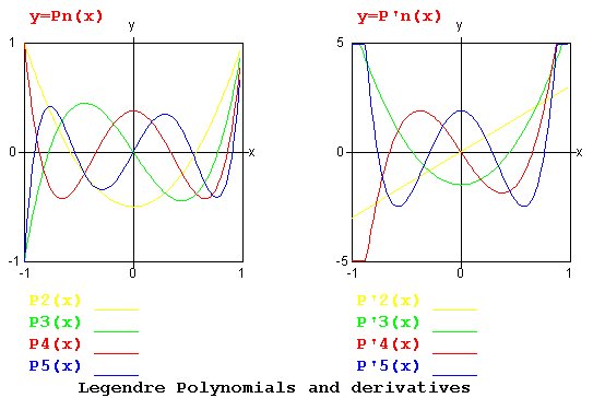
Chebyshev polynomials
T_n(x) are defined as
T_0(x) = 1
T_1(x) = x
T_2(x) = 2 x^2 - 1
T_3(x) = 4 x^3 - 3 x
T_4(x) = 8 x^4 - 8 x^2 + 1
the general recursion formula for T_n(x) is
T_n(x) = 2 x T_n-1(x) - T_n-2(x)
The weight function, w(x) = 1/sqrt(1-x^2)
The interval is a = -1 to b = 1
Explicit expression
T_n(x) = n/2 sum m=0 to n/2 (-1)^m (n-m-1)!/(m! (n-2m)!) (2x)^(n-2m)
T_n(x) = cos(n arccos(x))
Chebyshev polynomials are best known for approximating a function
while minimizing the maximum error, covered in a latter lecture.
Fit f(x) with approximate function F(x)
c_i = 2/pi integral x=-1 to 1 f(x) T_i(x) /sqrt(1-x^2) dx
(difficult near x=-1 and x=1)
F(x) = c_0 /2 + sum i=1 to n c_i T_i(x)
Change interval from t in [a, b] to x in [-1, 1]
x = (b+a+(b-a)t)/2
see example test program chebyshev.c
and results chebyshev_c.out
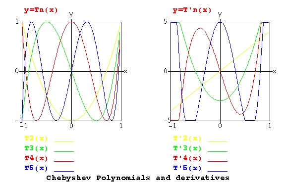
Laguerre polynomials
L_n(x) are defined as
L_0(x) = 1
L_1(x) = -x + 1
L_2(x) = x^2 - 4 x + 2
L_3(x) = -x^3 +9 x^2 - 18 x + 6
the general recursion formula for L_n(x) is
L_n(x) = (2n-x-1) L_n-1(x) - (n-1)^2 L_n-2(x)
The weight function, w(x) = e^(-x)
The interval is a = 0 to b = infinity
Explicit expression
L_n(x) = sum m=0 to n (-1)^m n!/(m! m! (n-m)!) x^m
L_n(x) = 1/(n! e^-x) d^n/dx^n (x^n e^(-x))
Laguerre polynomials are best known for use in integrating
functions where the upper limit is infinity.
Lagrange Polynomials
These will be used later in Galerkin Finite Element Method
for solving partial differential equations.
Lagrange polynomials L_n(x) are defined as
L_1,0(x) = 1 - x
L_1,1(x) = x
L_2,0(x) = 1 -3 x +2 x^2
L_2,1(x) = 4 x -4 x^2
L_2,2(x) = - x +2 x^2
L_3,0(x) = 1 -5.5 x +9 x^2 -4.5 x^3
L_3,1(x) = 9 x -22.5 x^2 +13.5 x^3
L_3,2(x) = -4.5 x +18 x^2 -13.5 x^3
L_3,3(x) = x -4.5 x^2 +4.5 x^3
L_4,1(x) = 16 x -69.33 x^2 + 96 x^3 - 42.33 x^4
L_5,2(x) = -25 x +222.92 x^2 -614.58 x^3 +677.08 x^4 -260.42 x^5
For 0 ≤ x ≤ 1 and equal spaced points in between.
The general recursion formula for L_n+1,j(x) is
unavailable
Explicit expression
L_n,k(x) = product i=0 to n, i/=k of (x-x_i)/(x_k-x_i)
Lagrange polynomials are best known for solving differential
equations with equal and unequal grid spacing.
An nth order Lagrange polynomial will exactly fit n data points.
Fit f(x) with approximate function F(x)
F(x) = sum k=0 to n of f(x_k) L_n,k(x)
Change of coordinates for integration
Change interval from t in [a, b] to x in [0, 1]
x = (t-a)/(b-a)
Change interval from t in [a, b] to x in [-1, 1]
x = 2(t-a)/(b-a)-1
Example plots
see example test program lagrange.c
and results lagrange_c.out
A family of Lagrange Polynomials can be constructed to be
1.0 at x_i and zero at every x_j where i ≠ j
Using the notation above, np=11 and each color is a different k.
Each of the 11 points has one color at 1.0 and all other
colors at 0.0 .
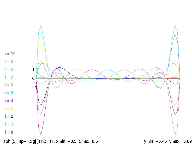 Lagrange Phi shape functions
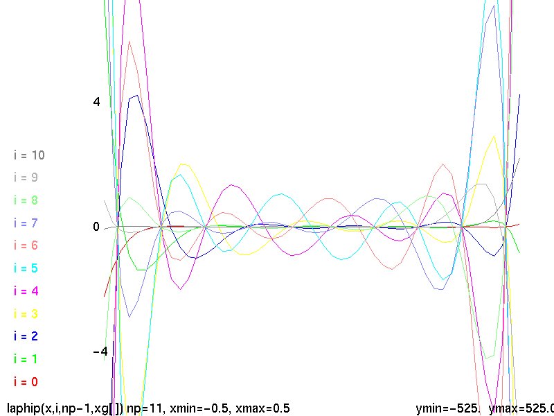 First derivative of Lagrange Phi shape functions
polynomial functions in python3
test_poly.py3 source code of functions
test_poly_py3.out output
test_poly2.py3 source code of functions
test_poly2_py3.out output
python3 divide integers produces floating point
test.py3 source code of functions
test_py3.out output
Additional utility functions:
cs455_l37.html
A function may be given as an analytic expression
such as sqrt(exp(x)-1.0) or may be given as a set
of points (x_i, y_i).
There are occasions when an efficient and convenient computer
implementation is needed. One of the efficient and convenient
implementations is a polynomial.
Thanks to Mr. Taylor and Mr. Maclaurin we can convert any
continuously differentiable function to a polynomial:
Taylor series, given differentiable function, f(x)
pick a convenient value for a
(x-a) f'(a) (x-a)^2 f''(a) (x-a)^3 f'''(a)
f(x) = f(a) + ----------- + -------------- + --------------- + ...
1! 2! 3!
Maclaurin series, same as Taylor series with a=0
x f'(0) x^2 f''(0) x^3 f'''(0)
f(x) = f(0) + ------- + ---------- + ----------- + ...
1! 2! 3!
Taylor series, function offset by value of h
h f'(x) h^2 f''(x) h^3 f'''(x)
f(x+h) = f(x) + ------- + ---------- + ----------- + ...
1! 2! 3!
Please use analytic differentiation rather than numerical differentiation.
Programs such as Maple have Taylor Series generation as a primitive.
An example Taylor series is: e^x = 1 + x + x^2/2! + x^3/3! + x^4/4!
Using a fixed number of terms, fourth power in this example,
will result in truncation error. The series has been truncated.
It should be obvious, that for large x, the error will become
very large. Also, this type of series will fail or be very
inaccurate if there are discontinuities in the function being fit.
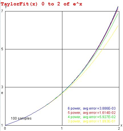
We often estimate "truncation" error as the next order term
that is not used.
Note the relation of "estimated truncation error" to maximum error
and rms error as more terms are used in the approximation.
TaylorFit.java
TaylorFit_java.out
It is interesting to note that: The truncation error is usually
slightly less than the maximum error, thus a reasonable estimate
of the accuracy of the fit.
Unequally spaced points often use least square fit
For functions given as unequally spaced points, use
the least square fit technique in Lecture 4
Fitting discontinuous data, try Fourier Series
For function with discontinuities the Fourier Series or
Fejer Series may produce the required fit.
The Fourier series approximation f(t) to f(x) is defined as:
f(t) = a_0/2 + sum n=1..N a_n cos(n t) + b_n sin(n t)
a_n = 1/Pi integral -Pi to Pi f(x) cos(n x) dx
b_n = 1/Pi integral -Pi to Pi f(x) sin(n x) dx
When given an analytic function, f(x) it may be best to use analytic
evaluation of the integrals. When given just points it may be best
to not use Fourier series, use Lagrange fit.
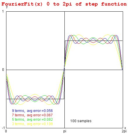 FourierFit.java
FourierFit.out
test_fourier.java source code
test_fourier_java.out output
test_fourier.dat for ploting
FourierFit.java
FourierFit.out
test_fourier.java source code
test_fourier_java.out output
test_fourier.dat for ploting
 test_fourier_fit.py3
test_fourier_fit_py3.out
test_fourier_fit.py3
test_fourier_fit_py3.out
 test_fourier_fit.py3
test_fourier_fit_py3.out
test_fourier_fit.py3
test_fourier_fit_py3.out
Smoothing discontinuous data with Fejer Series
The Fejer series approximation f(t) to f(x) is defined as:
f(t) = a_0/2 + sum n=1..N a_n (N-n+1)/N cos(n t) + b_n (N-n+1)/N sin(n t)
a_n = 1/Pi integral -Pi to Pi f(x) cos(n x) dx
b_n = 1/Pi integral -Pi to Pi f(x) sin(n x) dx
Basically the Fejer Series with the contribution of the higher
frequencies increased. This will give a smoother fit
with less oscillations. See plot for square wave.
 FejerFit.java
FejerFit.out
test_fejer.java source code
test_fejer_java.out output
test_fejer.dat for ploting
FejerFit.java
FejerFit.out
test_fejer.java source code
test_fejer_java.out output
test_fejer.dat for ploting
 FejerFit3.java
FejerFit3_java.out
FejerFit3.java
FejerFit3_java.out
 fejer_sqw.py3
fejer_sqw_py3.out
fejer_sqw.py3
fejer_sqw_py3.out
Lagrange Fit minimizes maximum error (at fit points)
The Lagrange Fit minimizes the error at the chosen points to fit.
The Lagrange Fit is good for fitting data given at uniform spacing.
The Lagrange fit requires the fewest evaluations of the function
to be fit, convenient if the function to be fit requires
significant computation time.
The Lagrange series approximation f(t) to f(x) is defined as:
L_n(x) = sum j=0..N f(x_j) L_n,j(x)
L_n,j(x) = product i=0..N i /= j (x - x_i)/(x_j - x_i)
Collect coefficients, a_n, of L_n(x) to get
f(t) = sum i=0..N a_n t^n
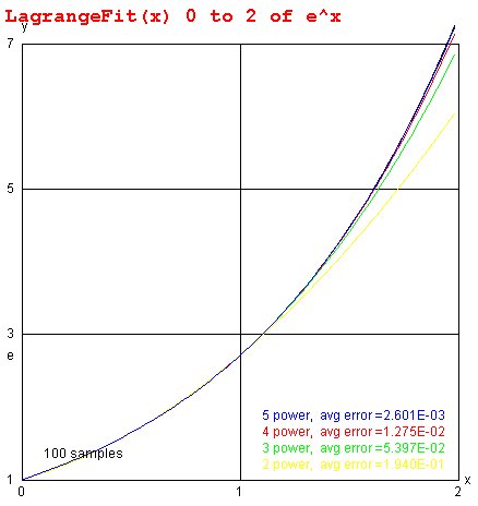 LagrangeFit.java
LagrangeFit.out
LagrangeFit.java
LagrangeFit.out
Legendre Fit minimizes RMS error
The Legendre Fit, similar to the Least Square Fit, minimizes
the RMS error of the fit.
The Legendre series approximation f(t) to f(x) is defined as:
f(t) = a_0 g_0 + sum n=1..N a_n g_n P_n(t) then combining coefficients can be
f(t) = sum n=0..n b_n t^n a simple polynomial
a_n = integral -1 to 1 f(x) P_n(x) dx
g_n = (2 n + 1)/2
P_0(x) = 1
P_1(x) = x
P_n(x) = (2n-1)/n x P_n-1(x) - (n-1)/n P_n-2(x)
Suppose f(x) is defined over the interval a to b, rather than -1 to 1, then
a_n = (b-a)/2 integral -1 to 1 f(a+b+x(b-a)/2) P_n(x) dx
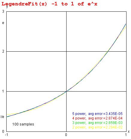 LegendreFit.java
LegendreFit.out
LegendreFit.java
LegendreFit.out
Chebyshev Fit minimizes maximum error (at fit points)
The Chebyshev Fit minimizes to maximum error of the fit for
a given order polynomial.
The Chebyshev series approximation f(t) to f(x) is defined as:
f(t) = a_0/2 + sum n=1..N a_n T_n(t) then combining coefficients can be
f(t) = sum n=0..n b_n t^n a simple polynomial
a_n = 2/Pi integral -1 to 1 f(x) T_n(x)/sqrt(1-x^2) dx
T_0(x) = 1
T_1(x) = x
T_n+1(x) = 2 x T_n(x) - T_n-1(x)
for -1 < x < 1 T_n(x) = cos(n acos(x))
When given an analytic function it may be best to use analytic
evaluation of the integrals. When given just points it may be best
to not use Chebyshev fit, use Lagrange fit. When given a
computer implementation of the function, f(x), to be fit,
use a very good adaptive integration.
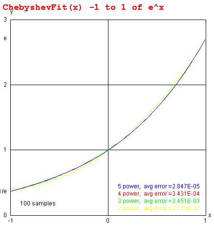 ChebyshevFit.java
ChebyshevFit.out
Note good intermediate points on smoth curve.
ChebyshevFit.java
ChebyshevFit.out
Note good intermediate points on smoth curve.
 test_chebyshev_fit.py3
test_chebyshev_fit_py3.out
Note bad intermediate points on square wave.
test_chebyshev_fit.py3
test_chebyshev_fit_py3.out
Note bad intermediate points on square wave.
 chebyshev_sqw.py3
Chebyshev_sqw_py3.out
chebyshev_sqw.py3
Chebyshev_sqw_py3.out
spline fit exact at data points with approximate slope
Involves computing derivatives and solving simultaneous equations
 Spline.java
Spline.out
SplineFrame.java
SplineFrame.out
SplineHelp.txt
SplineAbout.txt
SplineAlgorithm.txt
SplineIntegrate.txt
SplineEvaluate.txt
Source code and text output for the various fits:
LagrangeFit.java
LagrangeFit.out
LegendreFit.java
LegendreFit.out
FourierFit.java
FourierFit.out
FejerFit.java
FejerFit.out
ChebyshevFit.java
ChebyshevFit.out
You may convert any of these that you need to a language
of your choice.
learn language to convert to or from
Spline.java
Spline.out
SplineFrame.java
SplineFrame.out
SplineHelp.txt
SplineAbout.txt
SplineAlgorithm.txt
SplineIntegrate.txt
SplineEvaluate.txt
Source code and text output for the various fits:
LagrangeFit.java
LagrangeFit.out
LegendreFit.java
LegendreFit.out
FourierFit.java
FourierFit.out
FejerFit.java
FejerFit.out
ChebyshevFit.java
ChebyshevFit.out
You may convert any of these that you need to a language
of your choice.
learn language to convert to or from
Interactive Demonstration
Examples of interactive fitting of points may run:
java -cp . LeastSquareFitFrame
java -cp . LagrangeFitFrame
java -cp . SplineFrame
Lagrange.java
TestLagrange.java
TestLagrange.out
LagrangeFitFrame.java
LagrangeHelp.txt
LagrangeAbout.txt
LagrangeAlgorithm.txt
LagrangeIntegrate.txt
LagrangeEvaluate.txt
LeastSquareFit.java
LeastSquareFitFrame.java
LeastSquareFitHelp.txt
LeastSquareFitAbout.txt
LeastSquareFitAlgorithm.txt
LeastSquareFitIntegrate.txt
LeastSquareFitEvaluate.txt
Numerical Integration is usually called Numerical Quadrature.
Watch for "int" in this page it is short for "integrate".
Numerical integration could be simple summation, but
in order to get reasonable step size and good accuracy
we need better techniques.
integral f(x) dx from x=a to x=b with step size h=(b-a)/n
using simple summation would be computed:
area = (b-a)/n * ( sum i=0..n-1 f(a+i*h) ) not using f(b)
or
area = (b-a)/(n+1) * ( sum i=0..n f(a+i*h) )
"h" has become the approximation to "dx" using "n" steps.
A larger value of "n" gives a smaller value of "h" and
up to where round off error grows, a better approximation.
Shown is n=9 indicated by red dots.
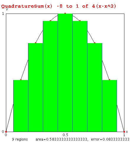 from QuadratureSum.java
Exact solution integral from 0 to 1 of 4(x-x^2) = 2/3 = 0.6666666
from QuadratureSum.java
Exact solution integral from 0 to 1 of 4(x-x^2) = 2/3 = 0.6666666
Trapezoidal method
The Trapezoidal rule approximates the area between x and x+h
as h * (f(x)+f(x+h))/2 , base times average height.
Summing the areas we note that f(a) and f(b) are used once
while the other intermediate f(x) are used twice, thus:
area = (b-a)/n * ( (f(a)+f(b))/2 + sum i=1..n-1 f(a+i*h) )
note: i=0 is f(a) i=n is f(b) thus sum index range 1..n-1
h = (b-a)/n
cutting h in half generally cuts the error in half for large n
Shown is n=8 regions based on 7 sums plus (f(a)+f(b))/2
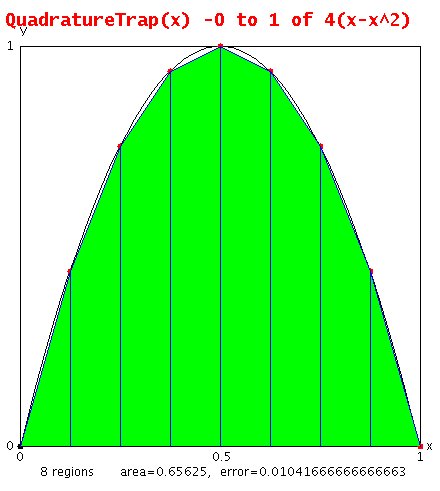 from QuadratureTrap.java
trapezoide.py Trapezoidal Integration
output is:
trapezoide.py running
trap_int area under x*x from 1.0 to 2.0 = 2.335
trapezoide.py finished
or trapezoide.py3 Trapezoidal Integration
trapezoide.java Trapezoidal Integration
output is:
trapezoide.java running
trap_int area under x*x from 1.0 to 2.0 = 2.3350000000000004
trapezoide.java finished
You do not need to use equal step sizes.
For better accuracy with trapazoidal integration,
use smaller step size where slope is largest.
Generally this requires more steps.
from QuadratureTrap.java
trapezoide.py Trapezoidal Integration
output is:
trapezoide.py running
trap_int area under x*x from 1.0 to 2.0 = 2.335
trapezoide.py finished
or trapezoide.py3 Trapezoidal Integration
trapezoide.java Trapezoidal Integration
output is:
trapezoide.java running
trap_int area under x*x from 1.0 to 2.0 = 2.3350000000000004
trapezoide.java finished
You do not need to use equal step sizes.
For better accuracy with trapazoidal integration,
use smaller step size where slope is largest.
Generally this requires more steps.
Better accuracy
In order to get better accuracy with fewer evaluations of
the function, f(x), we have found a way to choose the values
of x and to apply a weight, w(x) to each evaluation of f(x).
The integral is evaluated using:
area = sum i=1..n w(i)*f(x(i))
The w(i) and x(i) are computed using the Legendre polynomials
covered in the previous lecture. The numerical analysis shows
that using n evaluations we obtain accuracy about equal to
fitting the f(x(i)) with an nth order polynomial and accurately
computing the integral using that nth order polynomial.
Some values of weights w(i) and ordinates x(i) -1 < x < 1 are:
x[1]= 0.0000000000000E+00, w[1]= 2.0000000000000E+00
x[1]= -5.7735026918963E-01, w[1]= 1.0000000000000E-00
x[2]= 5.7735026918963E-01, w[2]= 1.0000000000000E-00
x[1]= -7.7459666924148E-01, w[1]= 5.5555555555555E-01
x[2]= 0.0000000000000E+00, w[2]= 8.8888888888889E-01
x[3]= 7.7459666924148E-01, w[3]= 5.5555555555555E-01
x[1]= -8.6113631159405E-01, w[1]= 3.4785484513745E-01
x[2]= -3.3998104358486E-01, w[2]= 6.5214515486255E-01
x[3]= 3.3998104358486E-01, w[3]= 6.5214515486255E-01
x[4]= 8.6113631159405E-01, w[4]= 3.4785484513745E-01
x[1]= -9.0617984593866E-01, w[1]= 2.3692688505618E-01
x[2]= -5.3846931010568E-01, w[2]= 4.7862867049937E-01
x[3]= 0.0000000000000E+00, w[3]= 5.6888888888889E-01
x[4]= 5.3846931010568E-01, w[4]= 4.7862867049937E-01
x[5]= 9.0617984593866E-01, w[5]= 2.3692688505618E-01
x[1]= -9.3246951420315E-01, w[1]= 1.7132449237916E-01
x[2]= -6.6120938646626E-01, w[2]= 3.6076157304814E-01
x[3]= -2.3861918608320E-01, w[3]= 4.6791393457269E-01
x[4]= 2.3861918608320E-01, w[4]= 4.6791393457269E-01
x[5]= 6.6120938646626E-01, w[5]= 3.6076157304814E-01
x[6]= 9.3246951420315E-01, w[6]= 1.7132449237916E-01
For a range from a to b, new_x[i] = a+(x[i]+1)*(b-a)/2
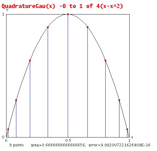 from QuadratureGau.java
and gauleg.java
Using the function gaulegf a typical integration could be:
double x[9], w[9] for 8 points
a = 0.5; integrate sin(x) from a to b
b = 1.0;
n = 8;
gaulegf(a, b, x, w, n); x's adjusted for a and b
area = 0.0;
for(j=1; j<=n; j++)
area = area + w[j]*sin(x[j]);
The following programs, gauleg for Gauss Legendre integration,
computes the x(i) and w(i) for various values of n. The
integration is tested on a constant f(x)=1.0 and then on
integral sin(x) from x=0.5 to x=1.0
integral exp(x) from x=0.5 to x=5.0
integral ((x^x)^x)*(x*(log(x)+1)+x*log(x)) from x=0.5 to x=5.0
This is labeled "mess" in output files.
Note how the accuracy increases with increasing values of n,
then, no further accuracy is accomplished with larger n.
Also note, the n where best numerical accuracy is achieved
is a far smaller n than where round off error would be
significant.
from QuadratureGau.java
and gauleg.java
Using the function gaulegf a typical integration could be:
double x[9], w[9] for 8 points
a = 0.5; integrate sin(x) from a to b
b = 1.0;
n = 8;
gaulegf(a, b, x, w, n); x's adjusted for a and b
area = 0.0;
for(j=1; j<=n; j++)
area = area + w[j]*sin(x[j]);
The following programs, gauleg for Gauss Legendre integration,
computes the x(i) and w(i) for various values of n. The
integration is tested on a constant f(x)=1.0 and then on
integral sin(x) from x=0.5 to x=1.0
integral exp(x) from x=0.5 to x=5.0
integral ((x^x)^x)*(x*(log(x)+1)+x*log(x)) from x=0.5 to x=5.0
This is labeled "mess" in output files.
Note how the accuracy increases with increasing values of n,
then, no further accuracy is accomplished with larger n.
Also note, the n where best numerical accuracy is achieved
is a far smaller n than where round off error would be
significant.
Downloadable code in C, Python, Fortran, Java, Ada and Matlab
Choose your favorite language and study the .out file
then look over the source code.
Just testing gaulegf:
integrate3d.java calculus
integrate3d_java.out numerical
gauleg.py function is gaulegf
test_gauleg.py
test_gauleg_py.out
gauleg.py3 function is gaulegf
test_gauleg.py3
test_gauleg_py3.out
gaulegf.java
test_gauleg.java
test_gauleg_java.out
gaulegf.h
gaulegf.c
test_gaulegf.c
test_gaulegf_c.out
test_gaulegf.cpp C++
test_gaulegf_cpp.out result
test_gaulegf.rb Ruby
test_gaulegf_rb.out result
gaulegf.adb
test_gaulegf.adb
test_gaulegf_ada.out
gaulegf.f90 original
Look near end of .out file, note convergence to exact value at end.
integral sin(x) from x=0.5 to x=1.0 for order 2 through 10
integral exp(x) from x=0.5 to x=5.0 for order 2 through 10
integral ((x^x)^x)*(x*(log(x)+1)+x*log(x)) from x=0.5 to x=5.0
This is labeled "mess" in output files. order 2 through 30
gauleg.c
gauleg_c.out
gauleg.f90
gauleg_f90.out
gauleg.for
gauleg_for.out
gauleg.java
gauleg_java.out
gauleg.adb
gauleg_ada.out
gaulegf.m
gauleg.m
gauleg_m.out
On Linux, you may use octave rather than MatLab.
Higher dimension, more independent variables
Multidimensional integration extends easily by using
gaulegf(ax, bx, xx, wx, nx); x's adjusted for ax and bx
gaulegf(ay, by, yy, wy, ny); y's adjusted for ay and by
volume = 0.0;
for(i=1; i<=nx; i++)
for(j=1; j<=ny; j++)
volume = volume + wx[i]*wy[j]*f(xx[i],yy[j]);
gaulegf(ax, bx, xx, wx, nx); x's adjusted for ax and bx
gaulegf(ay, by, yy, wy, ny); y's adjusted for ay and by
gaulegf(az, bz, zz, wz, nz); z's adjusted for az and bz
volume4d = 0.0;
for(i=1; i<=nx; i++)
for(j=1; j<=ny; j++)
for(k=1; k<=nz; k++)
volume4d = volume4d + wx[i]*wy[j]*wz[k]*f(xx[i],yy[j],zz[k]);
Volume code as shown in:
int2d.c
int2d_c.out
Additional reference books include:
"Handbook of Mathematical Functions" by Abramowitz and Stegun
A classic reference book on numerical integration and differentiation.
"Numerical Recipes in Fortran" by Press, Teukolsky, Vetterling and Flannery
There is also a "Numerical recipes in C" yet in my copy, there have
been a number of errors in the C code due to poor translation from Fortran.
Many very good numerical codes for general purpose and special purposes.
Integration of functions over triangles
An impressive example of quadrature over triangles is shown
by using Gauss Legendre integration coordinates rather than
splitting a triangle into smaller congruent triangles.
The routine "tri_split" converts a single triangle into four
congruent triangles that exactly cover the initial triangle.
Linear quadrature then uses just the center point of the
split, four equal area, triangles.
triquad.java triangle quadrature
test_triquad.java test
test_triquad.out results, see last two sets
Reducing the step size improves integration accuracy.
In two or more dimensions, reducing area, volume, etc.
improves integration accuracy. Two sets of triangle
splitting are shown below. Using higher order integration
provides more integration accuracy than smaller step size,
smaller area, volume, etc.
From tri_split.java
and test_tri_split.java
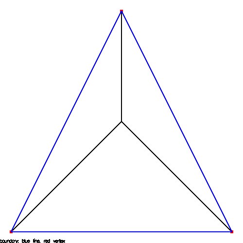
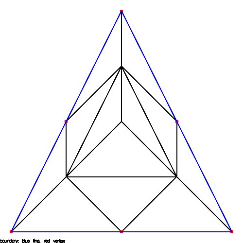
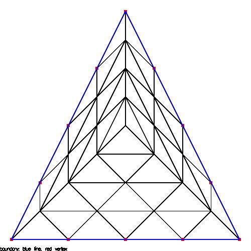
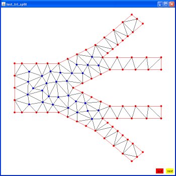
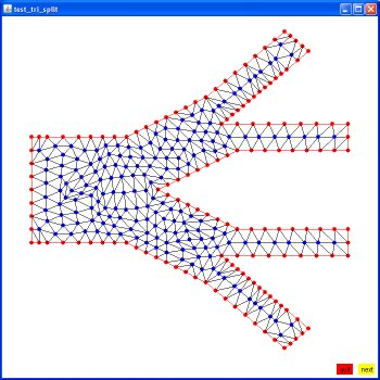
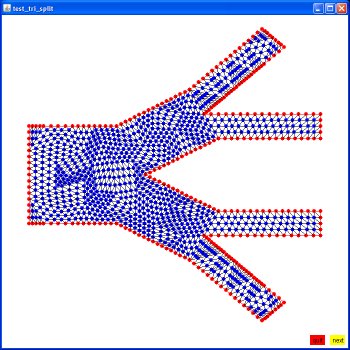 These will appear later in the solution of
partial differential equations using the Finite Element Method.
These will appear later in the solution of
partial differential equations using the Finite Element Method.
determine if a point is inside a polygon
point_in_poly.c
point_in_poly_c.out
point_in_poly.java
point_in_poly_java.out
Digitizing curves into computer
Scan the curve you want to digitize, sample curves listed below.
Compile Digitize.java
Run java Digitize your.jpg > your.out
Edit your.out to suit your needs. Output is scaled to your first 3 points.
(0,0) (1,0) (0,1)
Additional binary graphics files are:
pi.gif
curve.jpg
c6thrust.jpg
chess2.png
Digitize.out some output from curve.jpg
When working with calculus, you may encounter the "divergence theorem"
For a vector function F in a volume V with surface S
integrate over volume (∇˙F)dV =
integrate over surface (F˙normal)dS
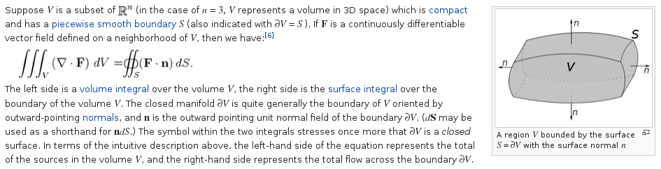 Just for fun, I programmed a numerical test to check the theorem
for one specific case: program and results of run
divergence_theorem.c
divergence_theorem_c.out
Just for fun, I programmed a numerical test to check the theorem
for one specific case: program and results of run
divergence_theorem.c
divergence_theorem_c.out
The general form of the trapezoidal integration.
a = integral y(x) dx over a set of increasing values of x, x_1 to x_n,
a = sum i=1 to i=n-1 of (x_i+1 - x_i) * (y(x_i) + y(x_i+1))/2
The (x_i+1 - x_i) is a variable version of h.
For best accuracy, pick x values where slope is changing,
in general use dx smaller for larger slope.
HW3 is assigned
When all else fails, there is adaptive numerical quadrature.
This is cleaver because the integration adjusts to the function
being integrated. And, yes, it can have problems.
The basic principle is to divide up the integration into
intervals. Use two methods of integration in each interval.
If the two methods do not agree in some interval, divide that
interval in half, and repeat. The total integral is the sum
of the integrals of all the intervals.
Consider integrating the function y = 1/x from 0.01 to 2.0,
with a high point at y=100 with a very steep slope and
a low relatively flat area from y=1.0 to y=0.5.
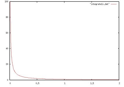 Note that the analytic solution is ln(2.0)-ln(0.01).
Do not try integration from 0 to 2, the integral is infinite.
The integral from 0.1 to 1 of 1/x = 2.302585093
The integral from 0.01 to 0.1 of 1/x = 2.302585093
The integral from 0.001 to 0.01 of 1/x = 2.302585093
Of course, ln(1)-ln(1/10) = 0 + ln(1/10) = 2.302585093
Thus, as we integrate closer and closer to zero, each factor
of 10 only adds 2.302585093 to the integral.
Note that the analytic solution is ln(2.0)-ln(0.01).
Do not try integration from 0 to 2, the integral is infinite.
The integral from 0.1 to 1 of 1/x = 2.302585093
The integral from 0.01 to 0.1 of 1/x = 2.302585093
The integral from 0.001 to 0.01 of 1/x = 2.302585093
Of course, ln(1)-ln(1/10) = 0 + ln(1/10) = 2.302585093
Thus, as we integrate closer and closer to zero, each factor
of 10 only adds 2.302585093 to the integral.
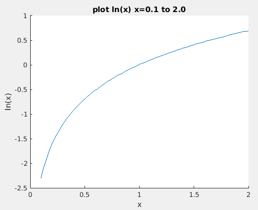 Here is a simple implementation of adaptive quadrature, in "C"
/* aquad.c adaptive quadrature numerical integration */
/* for a desired accuracy on irregular functions. */
/* define the function to be integrated as: */
/* double f(double x) */
/* { */
/* // compute value */
/* return value; */
/* } */
/* */
/* integrate from xmin to xmax */
/* approximate desired absolute error in all intervals, eps */
/* accuracy absolutely not guaranteed */
#undef abs
#define abs(x) ((x)<0.0?(-(x)):(x))
double aquad(double f(double x), double xmin, double xmax, double eps)
{
double area, temp, part, h;
double err;
int nmax = 2000;
double sbin[2000]; /* start of bin */
double ebin[2000]; /* end of bin */
double abin[2000]; /* area of bin , sum of these is area */
int fbin[2000]; /* flag, 1 for this bin finished */
int i, j, k, n, nn, done;
int kmax = 20; /* maximum number of times to divide a bin */
n=32; /* initial number of bins */
h = (xmax-xmin)/(double)n;
for(i=0; i<n; i++)
{
sbin[i] = xmin+i*h;
ebin[i] = xmin+(i+1)*h;
fbin[i] = 0;
}
k = 0;
done = 0;
nn = n; /* next available bin */
while(!done)
{
done = 1;
k++;
if(k>=kmax) break; /* quit if more than kmax subdivisions */
area = 0.0;
for(i=0; i<n; i++)
{
if(fbin[i]==1) /* this interval finished */
{
area = area + abin[i]; /* accumulate total area each pass */
continue;
}
temp = f((sbin[i]+ebin[i])/2.0); /* two integration methods */
part = f((3.0*sbin[i]+ebin[i])/4.0);
part = part + f((sbin[i]+3.0*ebin[i])/4.0);
abin[i] = (part+2.0*temp)*(ebin[i]-sbin[i])/4.0;
area = area + abin[i];
err = abs(temp-part/2.0);
if(err*1.414 < eps) /* heuristic */
{
fbin[i] = 1; /* this interval finished */
}
else
{
done = 0; /* must keep dividing */
if(nn>=nmax) /* out of space, quit */
{
done = 1;
for(j=i+1; j<n; j++) area = area + abin[j];
break; /* result not correct */
}
else /* divide interval into two halves */
{
sbin[nn] = (sbin[i]+ebin[i])/2.0;
ebin[nn] = ebin[i];
fbin[nn] = 0;
ebin[i] = sbin[nn];
nn++;
}
}
} /* end for i */
n = nn;
} /* end while */
return area;
} /* end aquad.c */
The results of integrating 1/x for various xmin to xmax are:
(This output linked with aquadt.c that has extra printout.)
test_aquad.c testing aquad.c 1/x eps=0.001
75 intervals, 354 funeval, 6 divides, small=0.101855, maxerr=0.000209298
xmin=0.1, xmax=2, area=2.99538, exact=2.99573, err=-0.000347413
261 intervals, 1470 funeval, 11 divides, small=0.0100607, maxerr=0.000228422
xmin=0.01, xmax=2, area=5.29793, exact=5.29832, err=-0.000390239
847 intervals, 4986 funeval, 16 divides, small=0.00100191, maxerr=0.000226498
xmin=0.001, xmax=2, area=7.6005, exact=7.6009, err=-0.000399734
2000 intervals, 9810 funeval, 18 divides, small=0.000100238, maxerr=0.0141083
xmin=0.0001, xmax=2, area=9.78679, exact=9.90349, err=-0.116702
2000 intervals, 9444 funeval, 17 divides, small=1.04768e-05, maxerr=49.455
xmin=1e-05, xmax=2, area=11.2703, exact=12.2061, err=-0.935768
1.0/((x-0.3)*(x-0.3)+0.01) + 1.0/((x-0.9)*(x-0.9)+0.04) -6
387 intervals, 2226 funeval, 6 divides, small=0.00390625, maxerr=0.000595042
xmin=0, xmax=1, area=29.8582, exact=29.8583, err=-0.000113173
test_aquad.c finished
Notice how the method failed with xmin=0.0001, maxed out on storage.
Yes, a better data structure would be a tree or linked list.
It can be made recursive yet that may not be a good idea.
(Programs die from stack overflow!)
On one case the adaptive quadrature used the bins shown in the figure:
Here is a simple implementation of adaptive quadrature, in "C"
/* aquad.c adaptive quadrature numerical integration */
/* for a desired accuracy on irregular functions. */
/* define the function to be integrated as: */
/* double f(double x) */
/* { */
/* // compute value */
/* return value; */
/* } */
/* */
/* integrate from xmin to xmax */
/* approximate desired absolute error in all intervals, eps */
/* accuracy absolutely not guaranteed */
#undef abs
#define abs(x) ((x)<0.0?(-(x)):(x))
double aquad(double f(double x), double xmin, double xmax, double eps)
{
double area, temp, part, h;
double err;
int nmax = 2000;
double sbin[2000]; /* start of bin */
double ebin[2000]; /* end of bin */
double abin[2000]; /* area of bin , sum of these is area */
int fbin[2000]; /* flag, 1 for this bin finished */
int i, j, k, n, nn, done;
int kmax = 20; /* maximum number of times to divide a bin */
n=32; /* initial number of bins */
h = (xmax-xmin)/(double)n;
for(i=0; i<n; i++)
{
sbin[i] = xmin+i*h;
ebin[i] = xmin+(i+1)*h;
fbin[i] = 0;
}
k = 0;
done = 0;
nn = n; /* next available bin */
while(!done)
{
done = 1;
k++;
if(k>=kmax) break; /* quit if more than kmax subdivisions */
area = 0.0;
for(i=0; i<n; i++)
{
if(fbin[i]==1) /* this interval finished */
{
area = area + abin[i]; /* accumulate total area each pass */
continue;
}
temp = f((sbin[i]+ebin[i])/2.0); /* two integration methods */
part = f((3.0*sbin[i]+ebin[i])/4.0);
part = part + f((sbin[i]+3.0*ebin[i])/4.0);
abin[i] = (part+2.0*temp)*(ebin[i]-sbin[i])/4.0;
area = area + abin[i];
err = abs(temp-part/2.0);
if(err*1.414 < eps) /* heuristic */
{
fbin[i] = 1; /* this interval finished */
}
else
{
done = 0; /* must keep dividing */
if(nn>=nmax) /* out of space, quit */
{
done = 1;
for(j=i+1; j<n; j++) area = area + abin[j];
break; /* result not correct */
}
else /* divide interval into two halves */
{
sbin[nn] = (sbin[i]+ebin[i])/2.0;
ebin[nn] = ebin[i];
fbin[nn] = 0;
ebin[i] = sbin[nn];
nn++;
}
}
} /* end for i */
n = nn;
} /* end while */
return area;
} /* end aquad.c */
The results of integrating 1/x for various xmin to xmax are:
(This output linked with aquadt.c that has extra printout.)
test_aquad.c testing aquad.c 1/x eps=0.001
75 intervals, 354 funeval, 6 divides, small=0.101855, maxerr=0.000209298
xmin=0.1, xmax=2, area=2.99538, exact=2.99573, err=-0.000347413
261 intervals, 1470 funeval, 11 divides, small=0.0100607, maxerr=0.000228422
xmin=0.01, xmax=2, area=5.29793, exact=5.29832, err=-0.000390239
847 intervals, 4986 funeval, 16 divides, small=0.00100191, maxerr=0.000226498
xmin=0.001, xmax=2, area=7.6005, exact=7.6009, err=-0.000399734
2000 intervals, 9810 funeval, 18 divides, small=0.000100238, maxerr=0.0141083
xmin=0.0001, xmax=2, area=9.78679, exact=9.90349, err=-0.116702
2000 intervals, 9444 funeval, 17 divides, small=1.04768e-05, maxerr=49.455
xmin=1e-05, xmax=2, area=11.2703, exact=12.2061, err=-0.935768
1.0/((x-0.3)*(x-0.3)+0.01) + 1.0/((x-0.9)*(x-0.9)+0.04) -6
387 intervals, 2226 funeval, 6 divides, small=0.00390625, maxerr=0.000595042
xmin=0, xmax=1, area=29.8582, exact=29.8583, err=-0.000113173
test_aquad.c finished
Notice how the method failed with xmin=0.0001, maxed out on storage.
Yes, a better data structure would be a tree or linked list.
It can be made recursive yet that may not be a good idea.
(Programs die from stack overflow!)
On one case the adaptive quadrature used the bins shown in the figure:
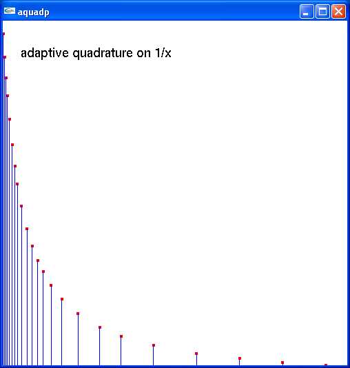 On some bigger problems, I had run starting with n = 8;
This missed the area where the slope was large.
Just like using the steepest descent method for finding roots,
you may hit a local flat area and miss the part that should
be adaptive.
The above was to demonstrate the "bins" and used way too much
memory. The textbook has pseudo code on Page 301 that uses
much less storage. A modified version of that code is:
/* aquad3.c from book page 301, with modifications */
#undef abs
#define abs(a) ((a)<0.0?(-(a)):(a))
static double stack[100][7]; /* a place to store/retrieve */
static int top, maxtop; /* top points to where stored */
void store(double s0, double s1, double s2, double s3, double s4,
double s5, double s6)
{
stack[top][0] = s0;
stack[top][1] = s1;
stack[top][2] = s2;
stack[top][3] = s3;
stack[top][4] = s4;
stack[top][5] = s5;
stack[top][6] = s6;
}
void retrieve(double* s0, double* s1, double* s2, double* s3, double* s4,
double* s5, double* s6)
{
*s0 = stack[top][0];
*s1 = stack[top][1];
*s2 = stack[top][2];
*s3 = stack[top][3];
*s4 = stack[top][4];
*s5 = stack[top][5];
*s6 = stack[top][6];
} /* end retrieve */
double Sn(double F0, double F1, double F2, double h)
{
return h*(F0 + 4.0*F1 + F2)/3.0; /* error term 2/90 h^3 f^(3)(c) */
} /* end Sn */
double RS(double F0, double F1, double F2, double F3,
double F4, double h)
{
return h*(14.0*F0 +64.0*F1 + 24.0*F2 + 64.0*F3 + 14.0*F4)/45.0;
/* error term 8/945 h^7 f^(8)(c) */
} /* end RS */
double aquad3(double f(double x), double xmin, double xmax, double eps)
{
double a, b, c, d, e;
double Fa, Fb, Fc, Fd, Fe;
double h1, h2, hmin;
double Sab, Sac, Scb, S2ab;
double tol; /* eps */
double val, value;
maxtop = 99;
top = 0;
value = 0.0;
tol = eps;
a = xmin;
b = xmax;
h1 = (b-a)/2.0;
c = a + h1;
Fa = f(a);
Fc = f(c);
Fb = f(b);
Sab = Sn(Fa, Fc, Fb, h1);
store(a, Fa, Fc, Fb, h1, tol, Sab);
top = 1;
while(top > 0)
{
top--;
retrieve(&a, &Fa, &Fc, &Fb, &h1, &tol, &Sab);
c = a + h1;
b = a + 2.0*h1;
h2 = h1/2;
d = a + h2;
e = a + 3.0*h2;
Fd = f(d);
Fe = f(e);
Sac = Sn(Fa, Fd, Fc, h2);
Scb = Sn(Fc, Fe, Fb, h2);
S2ab = Sac + Scb;
if(abs(S2ab-Sab) < tol)
{
val = RS(Fa, Fd, Fc, Fe, Fb, h2);
value = value + val;
}
else
{
h1 = h2;
tol = tol/2.0;
store(a, Fa, Fd, Fc, h1, tol, Sac);
top++;
store(c, Fc, Fe, Fb, h1, tol, Scb);
top++;
}
if(top>=maxtop) break;
} /* end while */
return value;
} /* end main of aquad3.c */
The same test cases, using aquad3t.c, gave the following result:
test_aquad3.c testing aquad3.c 1/x eps=0.001
aquad3 hitop=3, funeval=45, hmin=0.0148437
xmin=0.1, xmax=2, area=2.99573, exact=2.99573, err=9.25606e-07
aquad3 hitop=3, funeval=109, hmin=0.00048584
xmin=0.01, xmax=2, area=5.29832, exact=5.29832, err=1.50725e-06
aquad3 hitop=4, funeval=221, hmin=3.05023e-05
xmin=0.001, xmax=2, area=7.6009, exact=7.6009, err=1.65548e-06
aquad3 hitop=5, funeval=425, hmin=1.90725e-06
xmin=0.0001, xmax=2, area=9.90349, exact=9.90349, err=1.66753e-06
aquad3 hitop=6, funeval=777, hmin=1.19209e-07
xmin=1e-05, xmax=2, area=12.2061, exact=12.2061, err=1.66972e-06
1.0/((x-0.3)*(x-0.3)+0.01) + 1.0/((x-0.9)*(x-0.9)+0.04) -6
aquad3 hitop=5, funeval=121, hmin=0.0078125
xmin=0, xmax=1, area=29.8583, exact=29.8583, err=-1.6204e-06
test_aquad3.c finished
More accurate integration by yet another method:
This uses equally spaced points and gets more accuracy
by using more values of the function being integrated,
F0, F1, F2, ... (the first aquad above used h and 2h,
the aquad3 used 2h and 4h)
On some bigger problems, I had run starting with n = 8;
This missed the area where the slope was large.
Just like using the steepest descent method for finding roots,
you may hit a local flat area and miss the part that should
be adaptive.
The above was to demonstrate the "bins" and used way too much
memory. The textbook has pseudo code on Page 301 that uses
much less storage. A modified version of that code is:
/* aquad3.c from book page 301, with modifications */
#undef abs
#define abs(a) ((a)<0.0?(-(a)):(a))
static double stack[100][7]; /* a place to store/retrieve */
static int top, maxtop; /* top points to where stored */
void store(double s0, double s1, double s2, double s3, double s4,
double s5, double s6)
{
stack[top][0] = s0;
stack[top][1] = s1;
stack[top][2] = s2;
stack[top][3] = s3;
stack[top][4] = s4;
stack[top][5] = s5;
stack[top][6] = s6;
}
void retrieve(double* s0, double* s1, double* s2, double* s3, double* s4,
double* s5, double* s6)
{
*s0 = stack[top][0];
*s1 = stack[top][1];
*s2 = stack[top][2];
*s3 = stack[top][3];
*s4 = stack[top][4];
*s5 = stack[top][5];
*s6 = stack[top][6];
} /* end retrieve */
double Sn(double F0, double F1, double F2, double h)
{
return h*(F0 + 4.0*F1 + F2)/3.0; /* error term 2/90 h^3 f^(3)(c) */
} /* end Sn */
double RS(double F0, double F1, double F2, double F3,
double F4, double h)
{
return h*(14.0*F0 +64.0*F1 + 24.0*F2 + 64.0*F3 + 14.0*F4)/45.0;
/* error term 8/945 h^7 f^(8)(c) */
} /* end RS */
double aquad3(double f(double x), double xmin, double xmax, double eps)
{
double a, b, c, d, e;
double Fa, Fb, Fc, Fd, Fe;
double h1, h2, hmin;
double Sab, Sac, Scb, S2ab;
double tol; /* eps */
double val, value;
maxtop = 99;
top = 0;
value = 0.0;
tol = eps;
a = xmin;
b = xmax;
h1 = (b-a)/2.0;
c = a + h1;
Fa = f(a);
Fc = f(c);
Fb = f(b);
Sab = Sn(Fa, Fc, Fb, h1);
store(a, Fa, Fc, Fb, h1, tol, Sab);
top = 1;
while(top > 0)
{
top--;
retrieve(&a, &Fa, &Fc, &Fb, &h1, &tol, &Sab);
c = a + h1;
b = a + 2.0*h1;
h2 = h1/2;
d = a + h2;
e = a + 3.0*h2;
Fd = f(d);
Fe = f(e);
Sac = Sn(Fa, Fd, Fc, h2);
Scb = Sn(Fc, Fe, Fb, h2);
S2ab = Sac + Scb;
if(abs(S2ab-Sab) < tol)
{
val = RS(Fa, Fd, Fc, Fe, Fb, h2);
value = value + val;
}
else
{
h1 = h2;
tol = tol/2.0;
store(a, Fa, Fd, Fc, h1, tol, Sac);
top++;
store(c, Fc, Fe, Fb, h1, tol, Scb);
top++;
}
if(top>=maxtop) break;
} /* end while */
return value;
} /* end main of aquad3.c */
The same test cases, using aquad3t.c, gave the following result:
test_aquad3.c testing aquad3.c 1/x eps=0.001
aquad3 hitop=3, funeval=45, hmin=0.0148437
xmin=0.1, xmax=2, area=2.99573, exact=2.99573, err=9.25606e-07
aquad3 hitop=3, funeval=109, hmin=0.00048584
xmin=0.01, xmax=2, area=5.29832, exact=5.29832, err=1.50725e-06
aquad3 hitop=4, funeval=221, hmin=3.05023e-05
xmin=0.001, xmax=2, area=7.6009, exact=7.6009, err=1.65548e-06
aquad3 hitop=5, funeval=425, hmin=1.90725e-06
xmin=0.0001, xmax=2, area=9.90349, exact=9.90349, err=1.66753e-06
aquad3 hitop=6, funeval=777, hmin=1.19209e-07
xmin=1e-05, xmax=2, area=12.2061, exact=12.2061, err=1.66972e-06
1.0/((x-0.3)*(x-0.3)+0.01) + 1.0/((x-0.9)*(x-0.9)+0.04) -6
aquad3 hitop=5, funeval=121, hmin=0.0078125
xmin=0, xmax=1, area=29.8583, exact=29.8583, err=-1.6204e-06
test_aquad3.c finished
More accurate integration by yet another method:
This uses equally spaced points and gets more accuracy
by using more values of the function being integrated,
F0, F1, F2, ... (the first aquad above used h and 2h,
the aquad3 used 2h and 4h)
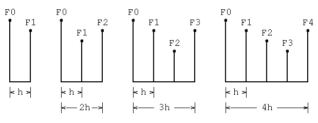 For case h, area = h(F0 + F1)/2
error = 1/12 h f''(c)
For case 2h, area = 2h(F0 + 4F1 + F2)/6
error = 2/90 h^3 f''''(c)
For case 3h, area = 3h(F0 + 3F1 + 3F2 + F3)/8
error = ? h^5 f'^(6)(c)
For case 4h, area = 4h(14F0 + 64F1 + 24F2 + 64F3 + 14F4)/180
error = 8/945 h^7 f'^(8)(c) eighth derivative, c is largest value
Then, the MatLab version:
% test_aquad.m 1/x eps = 0.001
function test_aquad
fid = fopen('test_aquad_m.out', 'w');
eps=0.001;
fprintf(fid, 'test_aquad.m running eps=%g\n', eps);
sprintf('generating test_aquad_m.out \n')
xmin = 0.1;
xmax = 2.0;
q = quad(@f,xmin,xmax,eps);
e = log(xmax)-log(xmin);
fprintf(fid,'xmin=%g, mmax=%g, area=%g, exact=%g, err=%g \n', xmin, xmax, e, q, e-q);
xmin = 0.01;
xmax = 2.0;
q = quad(@f,xmin,xmax,eps);
e = log(xmax)-log(xmin);
fprintf(fid,'xmin=%g, mmax=%g, area=%g, exact=%g, err=%g \n', xmin, xmax, e, q, e-q);
xmin = 0.001;
xmax = 2.0;
q = quad(@f,xmin,xmax,eps);
e = log(xmax)-log(xmin);
fprintf(fid,'xmin=%g, mmax=%g, area=%g, exact=%g, err=%g \n', xmin, xmax, e, q, e-q);
xmin = 0.0001;
xmax = 2.0;
q = quad(@f,xmin,xmax,eps);
e = log(xmax)-log(xmin);
fprintf(fid,'xmin=%g, mmax=%g, area=%g, exact=%g, err=%g \n', xmin, xmax, e, q, e-q);
xmin = 0.000001;
xmax = 2.0;
q = quad(@f,xmin,xmax,eps);
e = log(xmax)-log(xmin);
fprintf(fid,'xmin=%g, mmax=%g, area=%g, exact=%g, err=%g \n', xmin, xmax, e, q, e-q);
fprintf(fid,'1.0/((x-0.3)*(x-0.3)+0.01) + 1.0/((x-0.9).*(x-0.9)+0.04) -6\n');
xmin = 0.0;
xmax = 1.0;
q = quad(@f1,xmin,xmax,eps);
e = 29.8583;
fprintf(fid,'xmin=%g, mmax=%g, area=%g, exact=%g, err=%g \n', xmin, xmax, e, q, e-q);
fprintf(fid,'test_aquad.m finished\n');
return;
function y=f1(x)
y=1.0 ./ ((x-0.3) .*(x-0.3)+0.01) + 1.0 ./ ((x-0.9).*(x-0.9)+0.04) -6.0;
return
end
function y=f(x)
y = 1.0 ./ x;
return
end
end
with results:
test_aquad.m running eps=0.001
xmin=0.1, mmax=2, area=2.99573, exact=2.99597, err=-0.000241595
xmin=0.01, mmax=2, area=5.29832, exact=5.29899, err=-0.000668946
xmin=0.001, mmax=2, area=7.6009, exact=7.60218, err=-0.0012822
xmin=0.0001, mmax=2, area=9.90349, exact=9.90415, err=-0.000660689
xmin=1e-06, mmax=2, area=14.5087, exact=14.5101, err=-0.00148357
1.0/((x-0.3)*(x-0.3)+0.01) + 1.0/((x-0.9).*(x-0.9)+0.04) -6
xmin=0, mmax=1, area=29.8583, exact=29.8583, err=-8.17859e-06
test_aquad.m finished
The last case used the curve
y = 1.0/((x-0.3)*(x-0.3)+0.01) + 1.0/((x-0.9)*(x-0.9)+0.04) -6
that looks like:
For case h, area = h(F0 + F1)/2
error = 1/12 h f''(c)
For case 2h, area = 2h(F0 + 4F1 + F2)/6
error = 2/90 h^3 f''''(c)
For case 3h, area = 3h(F0 + 3F1 + 3F2 + F3)/8
error = ? h^5 f'^(6)(c)
For case 4h, area = 4h(14F0 + 64F1 + 24F2 + 64F3 + 14F4)/180
error = 8/945 h^7 f'^(8)(c) eighth derivative, c is largest value
Then, the MatLab version:
% test_aquad.m 1/x eps = 0.001
function test_aquad
fid = fopen('test_aquad_m.out', 'w');
eps=0.001;
fprintf(fid, 'test_aquad.m running eps=%g\n', eps);
sprintf('generating test_aquad_m.out \n')
xmin = 0.1;
xmax = 2.0;
q = quad(@f,xmin,xmax,eps);
e = log(xmax)-log(xmin);
fprintf(fid,'xmin=%g, mmax=%g, area=%g, exact=%g, err=%g \n', xmin, xmax, e, q, e-q);
xmin = 0.01;
xmax = 2.0;
q = quad(@f,xmin,xmax,eps);
e = log(xmax)-log(xmin);
fprintf(fid,'xmin=%g, mmax=%g, area=%g, exact=%g, err=%g \n', xmin, xmax, e, q, e-q);
xmin = 0.001;
xmax = 2.0;
q = quad(@f,xmin,xmax,eps);
e = log(xmax)-log(xmin);
fprintf(fid,'xmin=%g, mmax=%g, area=%g, exact=%g, err=%g \n', xmin, xmax, e, q, e-q);
xmin = 0.0001;
xmax = 2.0;
q = quad(@f,xmin,xmax,eps);
e = log(xmax)-log(xmin);
fprintf(fid,'xmin=%g, mmax=%g, area=%g, exact=%g, err=%g \n', xmin, xmax, e, q, e-q);
xmin = 0.000001;
xmax = 2.0;
q = quad(@f,xmin,xmax,eps);
e = log(xmax)-log(xmin);
fprintf(fid,'xmin=%g, mmax=%g, area=%g, exact=%g, err=%g \n', xmin, xmax, e, q, e-q);
fprintf(fid,'1.0/((x-0.3)*(x-0.3)+0.01) + 1.0/((x-0.9).*(x-0.9)+0.04) -6\n');
xmin = 0.0;
xmax = 1.0;
q = quad(@f1,xmin,xmax,eps);
e = 29.8583;
fprintf(fid,'xmin=%g, mmax=%g, area=%g, exact=%g, err=%g \n', xmin, xmax, e, q, e-q);
fprintf(fid,'test_aquad.m finished\n');
return;
function y=f1(x)
y=1.0 ./ ((x-0.3) .*(x-0.3)+0.01) + 1.0 ./ ((x-0.9).*(x-0.9)+0.04) -6.0;
return
end
function y=f(x)
y = 1.0 ./ x;
return
end
end
with results:
test_aquad.m running eps=0.001
xmin=0.1, mmax=2, area=2.99573, exact=2.99597, err=-0.000241595
xmin=0.01, mmax=2, area=5.29832, exact=5.29899, err=-0.000668946
xmin=0.001, mmax=2, area=7.6009, exact=7.60218, err=-0.0012822
xmin=0.0001, mmax=2, area=9.90349, exact=9.90415, err=-0.000660689
xmin=1e-06, mmax=2, area=14.5087, exact=14.5101, err=-0.00148357
1.0/((x-0.3)*(x-0.3)+0.01) + 1.0/((x-0.9).*(x-0.9)+0.04) -6
xmin=0, mmax=1, area=29.8583, exact=29.8583, err=-8.17859e-06
test_aquad.m finished
The last case used the curve
y = 1.0/((x-0.3)*(x-0.3)+0.01) + 1.0/((x-0.9)*(x-0.9)+0.04) -6
that looks like:
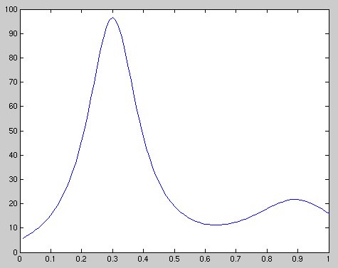 Passing a function as an argument in Python is easy:
# test_aquad3.py
from aquad3 import aquad3
xmin = 1.0
xmax = 2.0
eps = 0.001
def f(x):
return x*x
print "test_aquad3.py running"
area=aquad3(f, xmin, xmax, eps) # aquad3 compiled alone
print "aquad3(f, xmin, xmax, eps) =", area
With Java, some extra is needed to pass a user function to
a pre written integration class.
You need an interface to the function:
lib_funct.java
The user then provides an implementation to the function
to pass to the integration method and may provide values:
pass_funct.java
The pre written integration, trapezoidal method example,
has the numeric code, yet does not know the function (yet):
main_funct.java
main_funct.out
Then, a hack of test_aquad.c to test_aquad.java using just x^2
test_aquad.java
test_aquad_java.out
Another example with a two parameter function is:
(The Runga-Kutta method of integration is covered in Lecture 26.
This just shown the interface can be more general.)
You need an interface to the function:
RKlib.java
The user then provides an implementation to the function
to pass to the integration method and may provide values:
RKuser.java
The pre written integration method example,
has the numeric code, yet does not know the function (yet):
RKmain.java
RKmain.out
Passing a function as an argument in Python is easy:
# test_aquad3.py
from aquad3 import aquad3
xmin = 1.0
xmax = 2.0
eps = 0.001
def f(x):
return x*x
print "test_aquad3.py running"
area=aquad3(f, xmin, xmax, eps) # aquad3 compiled alone
print "aquad3(f, xmin, xmax, eps) =", area
With Java, some extra is needed to pass a user function to
a pre written integration class.
You need an interface to the function:
lib_funct.java
The user then provides an implementation to the function
to pass to the integration method and may provide values:
pass_funct.java
The pre written integration, trapezoidal method example,
has the numeric code, yet does not know the function (yet):
main_funct.java
main_funct.out
Then, a hack of test_aquad.c to test_aquad.java using just x^2
test_aquad.java
test_aquad_java.out
Another example with a two parameter function is:
(The Runga-Kutta method of integration is covered in Lecture 26.
This just shown the interface can be more general.)
You need an interface to the function:
RKlib.java
The user then provides an implementation to the function
to pass to the integration method and may provide values:
RKuser.java
The pre written integration method example,
has the numeric code, yet does not know the function (yet):
RKmain.java
RKmain.out
Now 3D integration
Matlab
integrate_volume.m source code
integrate_volume_m.out output
using different function definition format:
integrate_volume2.m source code
integrate_volume2_m.out output
Java very accurate using gaulegf
test_gaulegf3D.java source code
test_gaulegf3D_java.out output
Less accurate using trap and other methods
integrate_volume.java source code
integrate_volume_java.out output
integrate_volume.txt calculus
The files are:
test_aquad.c
aquad.h
aquad.c teaching version, do not use
aquadt.c
test_aquad_c.out
test_aquad3.c
aquad3.h
aquad3.c C implementation
test_aquad3_c.out
aquad3t.c
test_aquad3t_c.out
test_aquad.m MatLab builtin
test_aquad_m.out
test_aquad3.f90
aquad3.f90 Fortran 95 implementation
test_aquad3_f90.out
test_aquad3.adb
aquad.ads
aquad.adb Ada 95 implementation
f.adb
f1.adb
test_aquad3_ada.out
lib_funct.java
pass_funct.java
main_funct.java
test_aquad.java
test_aquad_java.out
test_passing_function.py
test_passing_function_py.out
test_aquad3.py
aquad3.py
test_aquad3_py.out
Go over WEB pages Lecture 1 through 8.
Work the homework 1 and homework 2.

Open book, open notes, exam.
Multiple choice and short answer.
Read the instructions.
Follow the instructions, else lose points.
Read the question carefully.
Answer the question that is asked, not the question you want to answer.
No programming required.
Some code may appear as part of a question.

Example questions and answers will be presented in class.
Some things you should know for the exam:

IEEE float has 6 or 7 decimal digits precision

IEEE double has 15 or 16 decimal digits precision

Adding or subtracting numbers of large differences in magnitude
causes precision lose. Known as roundoff error.

RMS error is root mean square error, a reasonable intuitive measure

Maximum error may be the most important measure for some applications

Average error is not very useful, typically smallest error.

The machine "epsilon" for a specific floating point arithmetic is
the smallest positive machine number added to exactly 1.0 that
results in a sum that is not exactly 1.0, actually greater than 1.0 .

Be careful reading programs that use "epsilon" or "eps". Sometimes
it may be the "machine epsilon" and other times it may be a
tolerance on how close the something should be.

Most languages include the elementary functions sin and cos, yet many
do not include a complete set of reciprocal functions such as cosecant
or inverse hyperbolic functions such as inverse hyperbolic cotangent.

If given only a natural logarithm function, log2(x) and be computed
as  log(x)/log(2.0) and log10(x) as log(x)/log(10.0)

Homework 1 used a simple approximation for integration:
position s = integral for time=0 to time=t of velocity(t) dt
as s = sum i=1 to n  s_i = s_i-1 + dv_i-1 * dt  where n*dt=t

In order to guarantee a mathematical unique solution to a set of
linear simultaneous equations, two requirements are needed:
There must be the same number of equations as unknown variables and
the equations must be linearly independent.

For two equations to be linearly independent, there must not be
two constants p and q such that equation1 * p + q = equation2

The numerical solution of liner simultaneous equations can fail even
though the mathematical condition for a unique solution exists.

Surprisingly, a good numerical solution usually results from
linear simultaneous equations based on random numbers.

The Gauss Jordan method of solving simultaneous equations A x = y produces
the solution x by performing operations on A y, reducing A to the
identity matrix such that y is replaced by x at the end of the computation

Improved numerical accuracy is obtained in the solution of linear
systems of equations by interchanging rows such that the largest
magnitude diagonal is used as the pivot element.
Some very large systems of equations can be solved accurately.

The system of linear equations is solved by the same method when
the equations have complex values.

It is better to directly solve simultaneous equations rather than
invert the "A" matrix and multiply by the "y" vector to find "x".
There are small matrices that are very hard to invert accurately.
Matrix inversion uses very similar computation to direct solving
of simultaneous equations. The matrix times vector, A * y, introduces
more error.

Given data, a least square fit of the data minimizes the RMS error
for a given degree polynomial at the data points. Between the
data points there may be large variations.

When trying to fit large degree polynomials, there may be numerical
errors such that the approximation becomes worse.

A polynomial of degree n, will exactly fit n+1 points.
It may have extreme humps and valleys between the points.

Mathematically, a least square fit of n data points should be
exactly fit by a n-1 degree polynomial. The numerical computation
may not give this result.

A least square fit may use terms: powers, sine, cosine or any other
smooth function of the data. The basic requirement is that
all functions must be linearly independent of each other.

A least square fit uses a solution of simultaneous equations

Least square fit is the easiest method of fitting data that
is given with unequal spacing.

A polynomial of degree n has n+1 coefficients. Thus n+1 data
points can be exactly fit by an n degree polynomial.

A polynomial of degree n has exactly n roots (possibly with multiplicity)

Given roots r1, r2, ... rn a polynomial with these roots is created by
(x-r1)*(x-r2)* ... *(x-rn)

Finding a root, r, divide the polynomial by (x-r) to reduce one degree.

Newton's method x_next = x - P(x)/P'(x) will have quadratic
convergence except near multiple roots or derivative P'(x)
small. An error of 1/16 will reduce to an error of 1/64
on the next iteration.

Horner's method of evaluating polynomials provides accuracy and
efficiency by never directly computing high powers of the variable.

Given the numerical coefficients of a polynomial, the numerical
coefficients of the integral, derivative are easily computed.

Given the numerical coefficients of two polynomials, the
sum, difference, product and ratio are easily computed.

Any functions that can be continuously differentiated can be
approximated by a Taylor series expansion. It is called
"truncation error" when evaluating a Taylor series with a
specific number of terms.

Orthogonal polynomials are used to fit data and perform numerical
integration. Examples of orthogonal polynomials include:
Legendre, Chebyshev, Laguerre, Lagrange, Fourier.

Chebyshev polynomials are used to approximate smooth functions
while minimizing the maximum error at the given data points.

Legendre polynomials are used to approximate smooth functions
while minimizing RMS error at the given data points.

Lagrange polynomials are used to approximate smooth functions
while exactly fitting the given data points.

For non smooth functions, including square waves and pulses,
a Fourier series approximation may be used.

The Fejer approximation can be used to eliminate many oscillations
in the Fourier approximation at the expense of a less accurate fit.

Numerical integration is typically called numerical quadrature.

The Trapezoidal integration method requires a small step size
and many function evaluations to get accuracy.
I used uniform step size and the method is easy to code:
area = (b-a)/n * ( (f(a)+f(b))/2 + sum i=1..n-1  f(a+i*h) )

In general a smaller the step size, usually called "h", will
result in a more accurate value for the integral. This
implies that more evaluations of the function to be
integrated are needed.

The Gauss Legendre integration of smooth functions provides
good accuracy with a minimum number of function evaluations.
The weights and ordinates are needed for the summation:
area = sum i=1..n  w[i]*f(x[i]);

An adaptive quadrature integration method is needed to
get reasonable accuracy of functions with large derivatives
or large variation in derivatives.

Adaptive quadrature uses a variable step size and at least
two methods of integration to determine when the desired
accuracy is achieved. This method, as with all integration
methods, can fail to give accurate results.

Two dimensional and higher dimensions can use simple extensions
of one dimensional numerical quadrature methods, except adaptive
quadrature.

The difference between a Taylor Series and a Maclaurin Series
is that the Maclaurin Series always expands a function about
zero.

The two equations for Standard Deviation are mathematically
equivalent, yet may give different numerical results.
sigma = sqrt((sum(x^2)- sum(x)^2/n)/n) = sqrt(sum((x-mean)^2)/n)
For n samples of x with a mean of mean.

RMS error is computed from a set of n error measurements using
rms_error = sqrt(sum(err^2)/n)
Note that this is the same value as Standard Deviation when
the mean value of the errors is zero. Thus, considered a
reasonable intuitive measure of error.
Multiple choice and short answer.
No help from other students, that is cheating!

The exam covers:
  lectures 1 through 9
  homework 1 and 2

sample quiz with sample answers for submit


Then on linux.gl.umbc.edu
  based on last name a-j a, m-r b, s-z c
  cp /afs/umbc.edu/users/s/q/squire/pub/download/q1_455a.doc
  cp /afs/umbc.edu/users/s/q/squire/pub/download/q1_455b.doc
  cp /afs/umbc.edu/users/s/q/squire/pub/download/q1_455c.doc

  Use Microsoft Word  or  libreoffice  to edit.

  submit cs455 quiz1 q1_455?.doc ? is a, b, or c


Download other files using the Linux  cp  command:
  Get any of my files you need on linux.gl.umbc.edu
  cp /afs/umbc.edu/users/s/q/squire/pub/download/some_file   .

  Be careful saving a file from a web page. You may have
  to fix broken lines.


quiz1 instructions for download:

quiz1 on homework page"
Then on linux.gl.umbc.edu
based on last name a-j a, m-r b, s-z c
cp /afs/umbc.edu/users/s/q/squire/pub/download/q1_455a.doc
cp /afs/umbc.edu/users/s/q/squire/pub/download/q1_455b.doc
cp /afs/umbc.edu/users/s/q/squire/pub/download/q1_455c.doc
Use Microsoft Word or libreoffice to edit.
submit cs455 quiz1 q1_455?.doc ? is a, b, or c
Download other files using the Linux cp command:
Get any of my files you need on linux.gl.umbc.edu
cp /afs/umbc.edu/users/s/q/squire/pub/download/some_file .
Be careful saving a file from a web page. You may have
to fix broken lines.
quiz1 instructions for download:
quiz1 on homework page"
There may be times when you have to do numerical computation
on complex values (scalars, vectors, or matrices).
If you are programming in Fortran, no problem, the types
complex and complex*16 or double complex are built in.
In Ada 95, the full set of complex arithmetic and functions
come with the compiler as packages. MatLab and Python use
complex as needed, automatically (e.g. output of FFT).
In other programming languages you need to know how to do
complex computation and how to choose the appropriate
numerical method.
older
C Java Fortran 95 Fortran Ada 95 MATLAB Python
------ ------ ---------------- ---------- ------------ -------- --------
complex
32 bit 'none' 'none' complex complex complex N/A N/A
64 bit 'none' 'none' double complex complex*16 long_complex 'default' 'default'
'none' means not provided by the language (may be available as a library)
N/A means not available, you get the default.
Background:
A complex number is stored in the computer as an ordered pair
of floating point numbers, the real part and the imaginary part.
The floating point numbers may be single or double precision as
needed by the application. It is suggested that you use double
precision as the default.
These are called Cartesian coordinates. Polar coordinates are
seldom used for computation, yet, are usually made available by
a conversion function to magnitude and angle. Note that
numerical analyst call the angle by the name "argument".
The naming convention depends on the programming language and
personal (or customer) choice.
Basic complex arithmetic is covered first and then complex
functions: sin, cos, tan, sinh, cosh, tanh, exp, log, sqrt, pow
are covered in the next lecture.
The simplest need for complex numbers is solving for the roots
of the polynomial equation x^2 + 1 = 0 .
There must be exactly two roots and they are sqrt(-1) and
-sqrt(-1) that are named "i" and "-i".
The quadratic equation for finding roots of a second order
polynomial should use the complex sqrt, even for real coefficients
a, b, and c, because the roots may be complex.
given: a x^2 + b x + c = 0 find the roots
b +/- sqrt(b^2 - 4 a c)
solution x = -----------------------
2 a
that computes complex roots if 4 a c > b^2
Of course, the equation correctly computes the roots when
a, b, and c are complex numbers.
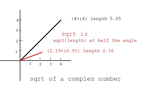
Complex Arithmetic
i=sqrt(-1) indicates imaginary part. a and b are real numbers.
(a+ib) is just two real numbers with b interpreted as imaginary.
Complex numbers are added by adding the real and imaginary parts:
(a+ib) + (c+id) = (a+c) + i(b+d)
Similarly, subtraction:
(a+ib) - (c+id) = (a-c) + i(b-d)
The multiplication of two complex numbers is:
(a+ib)*(c+id) = (a*c - b*d) + i(b*c + a*d)
The division of two complex numbers is:
r = c*c + d*d
(a+ib)/(c+id) = (a*c + b*d)/r + i(b*c - a*d)/r
Existing Implementations
The basic complex arithmetic (including some functions for
the next lecture) are in Complex.java
The automatically generated documentation is Complex.html
The complex arithmetic and functions in C uses "cx" named functions
as shown in the header file complex.h
and the body complex.c
with a test program test_complex.c
with results test_complex_c.out
The built in Ada package generic_complex_types.ads
provides complex arithmetic. Note the many operator definitions.
The use of complex in Ada is shown in this small program:
complx.adb
Complex functions are provided by generic_complex_elementary_functions.ads
The use of complex in Fortran 95 is shown in this small program:
complx.f90
C++ has the STL class Complex and can be used as shown
test_complex.cpp
test_complex_cpp.out
Python example
test_complex.py3
test_complex_py3.out
test_cxmath.py3
test_cxmath_py3.out
Cartesian Coordinates
Complex numbers define a plane and are typically Cartesian coordinates.
Polar coordinates also define a plane in terms of radius, r and angle θ.
x = r * cos(θ) r = sqrt(x*x+y*y)
y = r * sin(θ) θ = arctan(y/x) or atan2
Other coordinate systems are:
Cylindrical Coordinates
Cylindrical coordinates in terms of radius r, angle θ and height z.
x = r * cos(θ) r = sqrt(x*x+y*y)
y = r * sin(θ) θ = arctan(y/x) or atan2
z = z z = z
Spherical Coordinates
Spherical coordinates in terms of radius r, angles θ and φ
x = r * sin(φ) * cos(θ) r = sqrt(x*x+y*y+z*z)
y = r * sin(φ) * sin(θ) θ = arctan(y/x) or atan2
z = r * cos(φ) φ = arctan(sqrt(x*x+y*y)/z)
Toroidal Coordinates 1
The five independent variables are a, σ, θ, φ and z0
denom = cosh(θ)-cos(σ)
x = a * sinh(θ) * cos(φ) / denom
y = a * sinh(θ) * sin(φ) / denom
z = a * sin(σ) / denom optional + z0
-π < σ < π θ > 0 0 < φ < 2π a > 0
φ = arctan(y/x)
temporaries r1 = sqrt(x^2 + y^2)
d1 = sqrt((r1+a)^2 + z^2)
d2 = sqrt((r1-a)^2 + z^2)
θ = ln(d1/d2)
σ = arccos((d1^2+d2^2-4*a^2)/(2*d1*d2))
Toroidal Coordinates 2
The five independent variables are r1, r2, θ, φ, and z0
x = (r1 + r2 * sin(φ)) * cos(θ)
y = (r1 + r2 * sin(φ)) * sin(θ)
z = r2 * cos(φ) Optional + z0
0 < θ < 2π 0 < φ < 2π r1 > 0 r2 > 0
θ = arctan(y/x)
φ = arccos(z/r2)
r1 = x/cos(θ) - r2*sin(φ) or
r1 = y/sin(θ) - r2*sin(φ) no divide by zero
plot_toro.java try "run" etc
A simple implementation in C is demonstrated in
coordinate.c
coordinate.out
Beware of your choice of angle ranges when converting the above
radians to degrees.
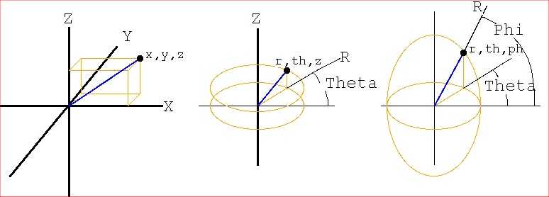 Cartesian Cylindrical Spherical
For Toroidal Coordinates 1:
toroidal_coord.c
toroidal_coord_c.out
toro.dat
toro.sh
toro.plot
Cartesian Cylindrical Spherical
For Toroidal Coordinates 1:
toroidal_coord.c
toroidal_coord_c.out
toro.dat
toro.sh
toro.plot
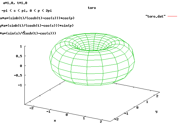 For Toroidal Coordinates 2:
toro2r.c
toro2r_c.out
toro2r.dat
toro2r.sh
toro2r.plot
For Toroidal Coordinates 2:
toro2r.c
toro2r_c.out
toro2r.dat
toro2r.sh
toro2r.plot
 or
toroidal1_coord.c
toroidal1_coord_c.out
toro1.dat
toro1.sh
toro1.plot
or
toroidal1_coord.c
toroidal1_coord_c.out
toro1.dat
toro1.sh
toro1.plot
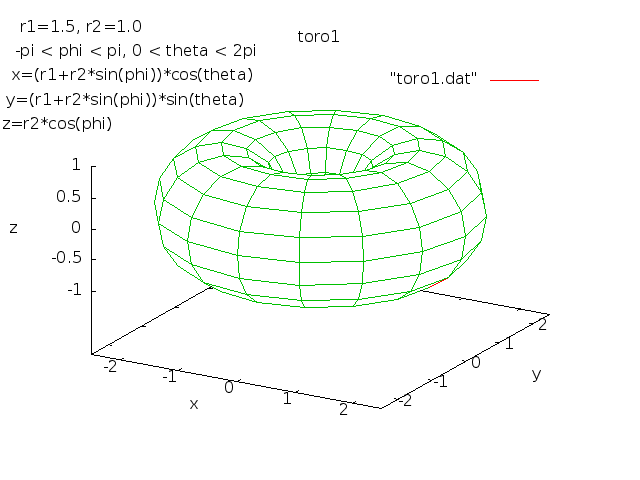 Then, for later, differential operators in three coordinate systems
del and other operators
Del_in_cylindrical_and_spherical_coordinates
Fast accurate numerical computing of derivatives and partial derivatives
is covered in
CS455 lecture 24 Derivatives
CS455 lecture 24a Partial Derivatives
If you need angles between vectors in two, three, four dimensions:
angle_vectors.py3 source code
angle_vectors_py3.out
Then, for later, differential operators in three coordinate systems
del and other operators
Del_in_cylindrical_and_spherical_coordinates
Fast accurate numerical computing of derivatives and partial derivatives
is covered in
CS455 lecture 24 Derivatives
CS455 lecture 24a Partial Derivatives
If you need angles between vectors in two, three, four dimensions:
angle_vectors.py3 source code
angle_vectors_py3.out
If you have code that works for double, extending to complex
may be easy.

Python evaluating a polynomial on "real" coefficients
  test_polyfit.py     polyfit in Python, needs numpy
from numpy import array
from numpy import polyfit
from numpy import polyval
import pylab

def f(x):
  return 5.0 + 4.0*x + 3.0*x*x + 2.0*x*x*x + 1.0*x*x*x*x

print "test_polyfit.py  a x,y,5) "
print "fit 5.0 + 4.0*x + 3.0*x*x + 2.0*x*x*x + 1.0*x*x*x*x"
xx = [0.0 for i in range(5)]
yy = [0.0 for i in range(5)]

for i in range(5):
  xx[i] = 0.1*(i+1)
  yy[i] = f(xx[i])    # function we will fit
  print "i=",
  print i,
  print " ,xx=",
  print xx[i],
  print " ,yy=",
  print yy[i]

print "p=polyfit(xx,yy,4) for 5 points"
p=polyfit(xx,yy,4) # 5 input values, 4th order
print "polyfit coefficients"
print p
print "backwards? largest power first, expected 5, 4, 3, 2, 1"
print " "
print "polyval values of fit"
yy1=polyval(p,xx)
print yy1
print "should be values above"
output
test_polyfit.py  a x,y,5)
fit 5.0 + 4.0*x + 3.0*x*x + 2.0*x*x*x + 1.0*x*x*x*x
i= 0  ,xx= 0.1  ,yy= 5.4321
i= 1  ,xx= 0.2  ,yy= 5.9376
i= 2  ,xx= 0.3  ,yy= 6.5321
i= 3  ,xx= 0.4  ,yy= 7.2336
i= 4  ,xx= 0.5  ,yy= 8.0625
p=polyfit(xx,yy,4) for 5 points
polyfit coefficients
[ 1.  2.  3.  4.  5.]
backwards? largest power first, expected 5, 4, 3, 2, 1

polyval values of fit
[ 5.4321  5.9376  6.5321  7.2336  8.0625]
should be values above

Python evaluating a polynomial on "complex" coefficients
  test_cxpolyfit.py     complex polyfit in Python, needs numpy
from numpy import array
from numpy import polyfit
from numpy import polyval
import pylab

def f(x): # changed to some complex coefficients
  return (5.0+1.0j) + (4.0+1.1j)*x + (3.0+1.2j)*x*x + 2.0*x*x*x + 1.0*x*x*x*x

print "test_cxpolyfit.py  a x,y,5) using complex numbers "
print "fit (5.0+1.0j) + (4.0+1.1j)*x + (3.0+1.2j)*x*x + 2.0*x*x*x + 1.0*x*x*x*x"
xx = [0.0 for i in range(5)]
yy = [0.0 for i in range(5)]

for i in range(5):
  xx[i] = 0.1*(i+1)
  yy[i] = f(xx[i])  # now has complex coefficients
  print "i=",
  print i,
  print " ,xx=",
  print xx[i],
  print " ,yy=",
  print yy[i]

print "p=polyfit(xx,yy,4) for 5 points"
p=polyfit(xx,yy,4) # 5 input values, 4th order
print "polyfit coefficients"
print p
print "backwards? largest power first, expected about 5, 4, 3, 2, 1"
print " "
print "polyval values of fit"
yy1=polyval(p,xx)
print yy1
print "should be values above"
output
test_cxpolyfit.py  a x,y,5) using complex numbers
fit (5.0+1.0j) + (4.0+1.1j)*x + (3.0+1.2j)*x*x + 2.0*x*x*x + 1.0*x*x*x*x
i= 0  ,xx= 0.1  ,yy= (5.4321+1.122j)
i= 1  ,xx= 0.2  ,yy= (5.9376+1.268j)
i= 2  ,xx= 0.3  ,yy= (6.5321+1.438j)
i= 3  ,xx= 0.4  ,yy= (7.2336+1.632j)
i= 4  ,xx= 0.5  ,yy= (8.0625+1.85j)
p=polyfit(xx,yy,4) for 5 points
polyfit coefficients
[ 1. +1.45680467e-12j  2. -1.77472663e-12j  3. +1.20000000e+00j
  4. +1.10000000e+00j  5. +1.00000000e+00j]
backwards? largest power first, expected about 5, 4, 3, 2, 1

polyval values of fit
[ 5.4321+1.122j  5.9376+1.268j  6.5321+1.438j  7.2336+1.632j  8.0625+1.85j ]
should be values above
No difference in polyfit or polyval, they accept real or complex.
 similar files to above
test_polyfit.py
test_polyfit_py.out
test_cxpolyfit.py
test_cxpolyfit_py.out

"C" language polyval on double
double polyval(int order, double p[], double x) // return y = p(x)
{             // using Horner's rule
  double y;
  int i;

  y = p[order]*x; // p one larger than order
  for(i=order-1; i>0; i--)
    y = (p[i]+y)*x;
  y = p[0]+y;
  return y;
} // end polyval
"C" language polyval on complex
easy editing a*b becomes cxmul(a,b)
             a+b becomes cxadd(a,b)
             double becomes complex
// #include "complex.h" compile with complex.c
complex cxpolyval(int order, complex p[], complex x) // return y = p(x)
{             // using Horner's rule
  complex y;
  int i;

  y = cxmul(p[order],x); // p one larger than order
  for(i=order-1; i>0; i--)
    y = cxmul(cxadd(p[i],y),x);
  y = cxadd(p[0],y);
  return y;
} // end cxpolyval

Java polyval on real
// polyval.java with simple test
class polyval
{
  polyval(){}

  double polyval(int order, double p[], double x) // return y = p(x)
  {             // using Horner's rule
    double y;
    y = p[order]*x; // p one larger than order
    for(int i=order-1; i>0; i--)
      y = (p[i]+y)*x;
    y = p[0]+y;
    return y;
  } // end polyval

  public static void main (String[] args)
  {
    double y;
    double x = 2.0;
    double p[] = {1.0, 2.0, 3.0};
    polyval c = new polyval();
    y = c.polyval(2, p, x);
    System.out.println("polyval.java on real");
    System.out.println("p = {"+p[0]+","+p[1]+","+p[2]+"}");
    System.out.println("y=p(x) x="+x+", y="+y);
  } // end main
} // end polyval.java
polyval.java real output
polyval.java on real
p = {1.0,2.0,3.0}
y=p(x) x=2.0, y=17.0

Java polyval on complex
easy editing a*b becomes a.multiply(b)
             a+b becomes a.add(b)
             double becomes Complex
// cxpolyval.java with simple test on Complex
// needs class Complex.class that defines type and functions
class cxpolyval
{
  cxpolyval(){}

  Complex cxpolyval(int order, Complex p[], Complex x) // return y = p(x)
  {             // using Horner's rule
    Complex y;
    y = p[order].multiply(x); // p one larger than order
    for(int i=order-1; i>0; i--)
	y = (p[i].add(y)).multiply(x);
    y = p[0].add(y);
    return y;
  } // end cxpolyval

  public static void main (String[] args)
  {
    Complex y;
    Complex x = new Complex(2.0, 0.1);
    Complex p[] = {new Complex(1.0,0.01), new Complex(2.0,0.02),
                   new Complex(3.0)};
    cxpolyval c = new cxpolyval();
    y = c.cxpolyval(2, p, x);
    System.out.println("cxpolyval.java on Complex");
    System.out.println("p = {"+p[0]+","+p[1]+","+p[2]+"}");
    System.out.println("y=p(x) x="+x+", y="+y);
  } // end main
} // end cxpolyval.java
cxpolyval.java complex output
cxpolyval.java on Complex
p = {(1.0,0.01),(2.0,0.02),(3.0,0.0)}
y=p(x) x=(2.0,0.1), y=(16.968,1.4500000000000002)

The notation (1.0,2.0) comes from Fortran where the
syntax was 1.0 real, 2.0 imaginary.

many Java files built for Complex
Complex.java
ComplexMatrix.java
ComplexPolynomial.java

Even least square fit can be performed on complex values
and the polynomial may have powers of all variables

 *    Y_actual         X1           X2
 *    --------       -----        -----
 *     32.5+i21.2    1.0+i1.0     2.5+i2.0
 *      7.2+i5.3     2.0+i1.1     2.5
 *      6.9+i1.1     3.0+i1.2     2.7
 *     22.4+i0.4     2.2+i2.2     2.1+i2.1
 *     10.4+i2.3     1.5+i3.4     2.0
 *     11.3+i4.0     1.6+i1.0     2.0
 *        ...          ...         ...  need at least as many as c's
 *
 *  Find coefficients c0, c1, c2, ...  such that
 *  Y_approximate =  c0 + c1*X1 + c2*X2 + c3*X1^2 + c4*X1*X2 + c5*X2^2 +
 *                   c6*X1^3 + c7*X1^2*X2 + c8*X1*X2^2 + c9*X2^3 + ...
 *  and such that the sum of (Y_actual - Y_approximate) squared is minimized.
 *  The same simultaneous equations are built, be sure to use a simultaneous
 *  equation solver where all arithmetic was changed to complex.

some examples with multiple variables to higher powers
(Sorry, modifying to complex is left as an exercise to the student.)
least_square_fit_2d.c
least_square_fit_3d.c
least_square_fit_4d.c
least_square_fit_4d.java
least_square_fit_4d_java.out
Some complex functions may be computed accurately from the basic
definition. But, preserving relative accuracy over the complete
domain of a few complex functions requires special techniques.
Note that the domain and range of complex functions may not be
obvious to the average user.
First, look at the mappings from domain z1 to range z2 for some
complex functions:
With Java applets enabled
If this does not work,
Complex Function Screen Shots
Various identities for elementary functions in the complex plane,
including implementing the complex function using only real functions.
Let z = x + i y
then arg z = arctan y/x real function using signs of x and y
modulus z = sqrt(x*x+y*y) = |z| length of complex vector
conjugate(z) = x - iy
re z = x
im z = y
SQRT
i (arg z)/2
sqrt z = sqrt(|z|) e
thus yielding half the angle with magnitude sqrt(|z|)
modulus z + re z modulus z - re z
sqrt z = sqrt ---------------- +/- i sqrt ----------------
2 2
where the sign of the imaginary part of the result is
the sign of the imaginary part of z
2 3
z z z
sqrt 1+z = 1 + - - -- + -- - ...
2 8 16
sqrt( 0 + i0) = 0 + i0
sqrt(-0 + i0) = 0 + i0
sqrt( 0 - i0) = 0 - i0
sqrt(-0 - i0) = 0 - i0
sqrt(z)**2 = z
sqrt(z*z) = z re z > 0
sqrt(1/z) = 1/sqrt(z) not for -0 or negative real axis
conjugate(sqrt(z)) = sqrt(conjugate(z)) not for -0 or negative real axis
Branch cut:
The branch cut lies along the negative real axis.
Domain:
Mathematically unbounded
Range:
Right half plane including the imaginary axis. The algebraic sign
of the real part is positive.
The sign of the imaginary part of the result is the same as the
sign of im z.
LOG
log z = ln( modulus z) + i argument z
2 3
z z
log 1+z = z - -- + -- - ... for |z| < 1
2 3
log(exp(z)) = z im z in [-Pi,Pi]
log(1/z) = -log(z) not on negative real axis
conjugate(log(z)) = log(conjugate(z)) not on negative real axis
Branch cut:
The branch cut lies along the negative real axis.
Domain:
Modulus z /= 0.0
Range:
Real part mathematically unbounded, imaginary part in range - Pi to Pi
The sign of the imaginary part of the result is the same as the
sign of im z.
EXP
z re z re z
e = e cos (im z) + i e sin (im z)
i x
e = cos(x) + i sin(x)
2 3
z z z
e = 1 + z + -- + -- + ...
2! 3!
z z+i 2Pi
e = e periodic with period i 2Pi
exp(-z) = 1/exp(z) not on negative real axis
exp(log(z)) = z |z| non zero
conjugate(exp(z)) = exp(conjugate(z))
Branch cut:
None
Domain:
re z < ln 'LARGE
Range:
Mathematically unbounded
For modulus z = 0.0, the result is 1.0 + z
"**"
w (w * ln z)
z = e
2 3
w (w ln z) (w ln z)
z = 1 + w ln z + --------- + --------- + ... for |z| non zero
2! 3!
w
log(z ) = w * log(z)
SIN
sin z = sin(re z) cosh(im z) + i cos(re z) sinh(im z)
iz -iz
e - e
sin z = -----------
2i
3 5
z z
sin z = z - -- + -- - ...
3! 5!
sin z = cos(z - Pi/2) periodic with period Pi
sin(z) = sin(z+2Pi)
sin z = -i sinh iz
sin(arcsin(z)) = z
sin(z) = -sin(-z)
conjugate(sin(z)) = sin(conjugate(z))
Domain:
|im z| < ln 'LARGE
COS
cos z = cos(re z) cosh(im z) - i sin(re z) sinh(im z)
iz -iz
e + e
cos z = -----------
2
2 4
z z
cos z = 1 - -- + -- - ...
2! 4!
cos z = sin(z + Pi/2) periodic with period Pi
cos(z) = cos(z+2Pi)
cos(z) = cos(-z)
cos z = cosh iz
cos(arccos(z)) = z
conjugate(cos(z)) = cos(conjugate(z))
Domain:
|im z| < ln 'LARGE
TAN
tan z = sin z / cos z
iz -iz
e - e
tan z = -i ---------- limit = -i when im z > ln 'LARGE
iz -iz limit = i when im z < - ln 'LARGE
e + e
3 5 7
z 2z 17z
tan z = z + -- + --- + ---- + ... for |z| < 1
3 15 315
sin x cos x sinh y cosh y
tan z = ---------------- +i ----------------
2 2 2 2
cos x + sinh y cos x + sinh y
tan z = cot(Pi/2 - z) periodic with period Pi
tan z = tan(z+2Pi)
tan z = 1/cot z
tan(z) = -tan(-z)
tan z = -i tanh iz
tan(arctan(z))=z
conjugate(tan(z)) = tan(conjugate(z))
Branch cut:
None
Domain:
Mathematically unbounded
Range:
Mathematically unbounded
For modulus z = 0.0, the result is z
COT
cot z = cos z / sin z
iz -iz
e + e
cot z = i ---------- limit = i when im z > ln 'LARGE
iz -iz limit = -i when im z < -ln 'LARGE
e - e
sin x cos x sinh y cosh y
cot z = ---------------- -i ----------------
2 2 2 2
sin x + sinh y sin x + sinh y
3 5
1 z z 2z
cot z = - - - - -- - --- - ...
z 3 45 945
cot z = tan(Pi/2 - z) periodic with period Pi
cot(z) = cot(z+2Pi)
cot(z) = -cot(-z)
cot z = 1/tan z
conjugate(cot(z)) = cot(conjugate(z))
Branch cut:
None
Domain:
Mathematically unbounded
Range:
Mathematically unbounded
For modulus z = 0.0, the result is z
ARCSIN
2
arcsin z = - i ln(i z + sqrt(1-z ))
arcsin z = - i ln(i z + sqrt(1-z)*sqrt(1+z))
3 5 7
z 3z 5z
arcsin z = z + -- + --- + ---- + ... for |z| < 1
6 40 112
1 3 15
arcsin z = -i( ln(2iz) - --- - ---- - ----- - ... ) for |z| > 1
2 4 6
4z 32z 288z
2
arcsin z = arctan(z/sqrt(1-z )) fix re of result
arcsin z =
2 2 1/2 2 2 1/2
arcsin(1/2 (x + 2 x + 1 + y ) - 1/2 (x - 2 x + 1 + y ) )
+ i
2 2 1/2 2 2 1/2
csgn(-i x + y) ln(1/2 (x + 2 x + 1 + y ) + 1/2 (x - 2 x + 1 + y )
2 2 1/2 2 2 1/2 2 1/2
+ ((1/2 (x + 2 x + 1 + y ) + 1/2 (x - 2 x + 1 + y ) ) - 1) )
note: The csgn function is used to determine in which half-plane
(`left' or `right') the complex-valued expression
or number x lies. It is defined by
/ 1 if Re(x) > 0 or Re(x) = 0 and Im(x) > 0
csgn(x) = < -1 if Re(x) < 0 or Re(x) = 0 and Im(x) < 0
\ 0 if x = 0
arcsin z = pi/2 - arccos z
arcsin z = -i arcsinh iz
arcsin(sin(z)) = z
Branch cut:
The real axis not in [ -1.0, 1.0 ]
Domain:
Mathematically unbounded
Range:
Imaginary part mathematically unbounded, real part in [ -Pi/2, Pi/2 ]
For modulus z = 0.0, the result is z
ARCCOS
1+z 1-z
arccos z = -i 2 ln( sqrt --- +i sqrt --- )
2 2
2
arccos z = -i ln(z + i sqrt(1-z ) )
3 5
Pi z 3z
arccos z = -- - z - -- - -- - ... for |z| < 1
2 6 40
arccos z = -i( ln(2z) for |z| > 1/sqrt(epsilon)
arccos z =
2 2 1/2 2 2 1/2
arccos(1/2 (x + 2 x + 1 + y ) - 1/2 (x - 2 x + 1 + y ) )
+ i
2 2 1/2 2 2 1/2
csgn(I x - y) ln(1/2 (x + 2 x + 1 + y ) + 1/2 (x - 2 x + 1 + y )
2 2 1/2 2 2 1/2 2 1/2
+ ((1/2 (x + 2 x + 1 + y ) + 1/2 (x - 2 x + 1 + y ) ) - 1) )
2
arccos z = arctan(sqrt(1-z )/z) fix re of result
arccos z = pi/2 - arcsin z
arccos(cos(z)) = z
Branch cut:
The real axis not in [ -1.0, 1.0 ]
Domain:
Mathematically unbounded
Range:
Imaginary part mathematically unbounded, real part in [ 0.0, Pi ]
ARCTAN
arctan z = -i ( ln(1 + i z) - ln(1 - i z) )/2
i i+z
arctan z = - ln --- must be fixed on slit for iz < -1
2 i-z
3 5 7
z z z
arctan z = z - -- + -- - -- + ... for |z| < 1
3 5 7
arctan z = Pi/2 - arccot z
arctan z = arccot(1/z)
arctan z = -i arctanh iz
arctan(tan(z)) = z
arctan z = 1/2 arctan(x, 1 - y) - 1/2 arctan(- x, y + 1)
2 2
x + (y + 1)
+i 1/4 ln(-------------)
2 2
x + (y - 1)
ARCCOT
i z-i
arccot z = - ln ---
2 z+i
3 5
Pi z z
arccot z = -- - z + -- - -- + ... for |z| < 1
2 3 5
arccot z = Pi/2 - arctan z
arccot z = arctan(1/z)
arccot(cot(z)) = z
arccot z = 1/2 Pi - 1/2 arctan(x, 1 - y) + 1/2 arctan(- x, y + 1)
2 2
x + (y + 1)
-i 1/4 ln(-------------)
2 2
x + (y - 1)
Range:
Imaginary part mathematically unbounded, real part in [0.0 , Pi]
SINH
sinh z = sinh(re z) cos(im z) + i cosh(re z) sin(im z)
z -z
e - e
sinh z = --------
2
3 5
z z
sinh z = z + -- + -- + ...
3! 5!
sinh z = -i cosh(z +i Pi/2) periodic with period i Pi
sinh z = -i sin iz
COSH
cosh z = cosh(re z) cos(im z) + i sinh(re z) sin(im z)
z -z
e + e
cosh z = --------
2
2 4
z z
cosh z = 1 + -- + -- + ...
2! 4!
cosh z = -i sinh(z +i Pi/2) periodic with period i Pi
cosh z = cos iz
TANH
tanh z = sinh z / cosh z
z -z
e - e
tanh z = --------
z -z
e + e
3 5 7
z 2z 17z
tanh z = z - -- + -- - ---- + ... for |z| < 1
3 15 315
tanh z = -i coth(z +i Pi/2) periodic with period i Pi
tanh z = 1/coth z
tanh z = -i tan iz
sinh x cosh x sin y cos y
tanh z = ---------------- +i ----------------
2 2 2 2
sinh x + cos y sinh x + cos y
COTH
coth z = cosh z / sinh z
z -z
e + e
coth z = --------
z -z
e - e
3 5
1 z z 2z
coth z = - + - - -- + --- - ... for |z| < 1
z 3 45 945
coth z = -i tanh(z +i Pi/2)
coth z = 1/tanh z
sinh x cosh x sin y cos y
coth z = ---------------- -i ----------------
2 2 2 2
sinh x + sin y sinh x + sin y
ARCSINH
2
arcsinh z = ln(z + sqrt(1 + z ) )
3 5 7
z 3z 5z
arcsinh z = z - -- + --- - --- + ... for |z| < 1
6 40 112
1 3 15
arcsinh z = ln(2z) + --- - ---- + ----- - ... for |z| > 1
2 4 6
4z 32z 288z
arcsinh z = -i arcsin iz
arcsinh(sinh(z)) = z
arcsinh z =
2 2 1/2 2 2 1/2
csgn(x + I y) ln(1/2 (x + y + 2 y + 1) + 1/2 (x + y - 2 y + 1)
2 2 1/2 2 2 1/2 2 1/2
+ ((1/2 (x + y + 2 y + 1) + 1/2 (x + y - 2 y + 1) ) - 1) )
+ i
2 2 1/2 2 2 1/2
arcsin(1/2 (x + y + 2 y + 1) - 1/2 (x + y - 2 y + 1) )
ARCCOSH
z+i z-i
arccosh z = 2 ln( sqrt --- + sqrt --- )
2 2
arccosh z = ln(z + sqrt(z-1) sqrt(z+1) ) not sqrt(z**2-1)
1 3 15
arccosh z = ln(2z) - --- - ---- - ----- - ... for |z| > 1
2 4 6
4z 32z 288z
arccosh(cosh(z)) = z
arccosh z =
2 2 1/2
- csgn(I - I x + y) csgn(I x - y) ln(1/2 (x + 2 x + 1 + y )
2 2 1/2
+ 1/2 (x - 2 x + 1 + y )
2 2 1/2 2 2 1/2 2 1/2
+ ((1/2 (x + 2 x + 1 + y ) + 1/2 (x - 2 x + 1 + y ) ) - 1) )
+ i
csgn(I - I x + y)
2 2 1/2 2 2 1/2
arccos(1/2 (x + 2 x + 1 + y ) - 1/2 (x - 2 x + 1 + y ) )
ARCTANH
arctanh z = ( ln(1+z) - ln(1-z) )/2
1 1+z
arctanh z = - ln --- must fix up on slit for z > 1
2 1-z
3 5 7
z z z
arctanh z = z + -- + -- + -- + ... for |z| < 1
3 5 7
arctanh z = -i arctan iz
arctanh(tanh(z)) = z
arctanh z = arccoth(z) + i Pi/2
2 2
(x + 1) + y
arctanh z = 1/4 ln(-------------)
2 2
(x - 1) + y
+i 1/2 arctan(y, x + 1) - 1/2 arctan(- y, 1 - x)
ARCCOTH
1 z+1
arccoth z = - ln --- must fix up on slit
2 z-1
3 5
i Pi z z
arccoth z = ---- + z + -- + -- + ... for |z| < 1
2 3 5
arccoth z = arctanh(z) +i Pi/2
arccoth z = arctanh(1/z)
arccoth(coth(z)) = z
2 2
(x + 1) + y
arccoth z = 1/4 ln(-------------)
2 2
(x - 1) + y
+i 1/2 Pi + 1/2 arctan(y, x + 1) - 1/2 arctan(- y, 1 - x)
Range:
Real part mathematically unbounded, imaginary part in [0.0 , i Pi]
There are many complex functions provided by Ada
generic_complex_elementary_functions.ads
Fortran 90 has a few complex functions
complex_func.f90 source code
complex_func_f90.out output
Python has many complex functions
test_complex.py3 source code
test_complex_py3.out output
Haskell has many complex functions
test_complex.hs source code
test_complex_hs.out output
Complex.hs Library module
I programmed some complex functions and utility routines in java.
Complex.java source code
TestComplex.java source code test
TestComplex_java.out output
Csimeq.java source code
test_Csimeq.java source code test
test_Csimeq_java.out test output
Cinvert.java source code
test_Cinvert.java source code test
test_Cinvert_java.out test output
Cnuderiv.java source code
test2_Cnuderiv.java source code test
test2_Cnuderiv_java.out test output
I programmed some complex functions and utility routines in ballerina.
complex_math.bal source code
complex_math_bal.out test output
Solving PDE with Complex functions, Complex solutions and Complex boundaries:
First the real, double, version second order, two dimensions
pdenu22_eq.java real source code test
pdenu22_eq_java.out test output
Then, converted to complex, Complex, version (using utilities above)
pdeCnu22_eq.java Complex source code test
pdeCnu22_eq_java.out test output
First the real, double, version fourth order, four dimensions
pde44h_eq.java real source code test
pde44h_eq_java.out test output
Then, converted to complex, Complex, version (using utilities above)
pdeC44h_eq.java Complex source code test
pdeC44h_eq_java.out test output
A much easier conversion to complex in Fortran
simeqC.f90 complex source code
inverseC.f90 complex source code
nuderivC.f90 complex source code
nuderivC_test.f90 complex source code
nuderivC_test_f90.out test output
pdeC44h_eq.f90 Complex source code test
pdeC44h_eq_f90.out test output
Similar maximum errors in real and complex code
MatLab overloads all functions that take floating point
to also work with complex numbers.
Python need to use cmath.
Eigenvalue and Eigenvector computation may be the most prolific for
special case numerical computation. Considering the size and speed
of modern computers, I use a numerical solution for a general
complex matrix. Thus, I do not have to worry about the constraints
on the matrix (is it numerically positive definite?)
The eigenvalues of a matrix with only real elements may be complex.
| 2.0 -2.0 |
| 1.0 0.0 | has eigenvalues 1+i and 1-i
Thus, computing eigenvalues needs to use complex arithmetic.
This type of numerical algorithm, you do not want to develop yourself.
The technique is to find a working numerical code, test it yourself,
then adapt the code to your needs, possibly converting the code to
a different language.
Eigenvalues have application in the solution of some physics problems.
They are also used in some solutions of differential equations.
Some statistical analysis uses eigenvalues. Sometimes only the
largest or second largest eigenvalues are important.
My interest comes from the vast types of testing that can, and should,
be performed on any code that claims to compute eigenvalues and
eigenvectors. Thorough testing of any numeric code you are going
to use is essential.
Information about eigenvalues, e (no lambda in plain ASCII)
and eigenvectors, v, for arbitrary n by n complex matrix A.
There are exactly n eigenvalues (some may have multiplicity greater than 1)
For every eigenvalue there is a corresponding eigenvector.
For eigenvalues with multiplicity greater than 1,
each has a unique eigenvector.
The set of n eigenvectors form a basis, they are all mutually orthogonal.
(The dot product of any pair of eigenvectors is zero.)
View this page in a fixed width font, else the matrices are shambles.
Vertical bars, | |, in this lecture is not absolute value,
it means vector or matrix
| 1 0 0 |
det|A-eI| = 0 defines e, where I is an n by n identity matrix | 0 1 0 |
zero except 1 on the diagonal | 0 0 1 |
(n e's for n by n A)
For a 3 by 3 matrix A:
| a11-e a12 a13 |
det| a21 a22-e a23 | = (a11-e)*(a22-e)*(a33-e)+a12*a23*a31+a13*a32*a21-
| a31 a32 a33-e | a31*(a22-e)*a13-a21*a12*(a33-e)-a32*a23*(a11-e)
Writing out the above determinant gives the "Characteristic Equation"
of the matrix A.
Combining terms gives e^n + c_n-1 * e^n-1 + ... + c_2 * e^2 + c_1 * e + c_0 = 0
(Divide through by c_n, to have exactly n unknown coefficients 0..n-1).
(Special case because of " = 0 " )
There are exactly n roots for an nth order polynomial and the
n roots of the characteristic equation are the n eigenvalues.
The relation between each eigenvalue and its corresponding eigenvector is
Av = ev where |v| is non zero.
Typically, we require the length of v to be 1.
Given a matrix A and a non singular matrix P and P inverse p^-1
B = P A P^-1 the matrix B has the same eigenvalues as matrix A.
The eigenvectors may be different.
B is a similarity transform of A.
The diagonal elements of a diagonal matrix are the eigenvalues of the matrix.
| a11 0 0 0 |
| 0 a22 0 0 |
| 0 0 a33 0 | has eigenvalues a11, a22, a33, a44 and
| 0 0 0 a44 |
corresponding eigenvectors
v1=|1 0 0 0| v2=|0 1 0 0| v3=|0 0 1 0| v4=|0 0 0 1|
Notice that the eigenvectors are not necessarily unique and may be
scaled by an arbitrary, non zero, constant. Normalizing the length
of each eigenvector to 1.0 is common.
The eigenvalues of a 2 by 2 matrix are easily computed as the roots
of a second order equation.
det| a11-e a12 |=0 or (a11-e)*(a22-e) - a12*a21 = 0 or
| a21 a22-e |
e^2 - (a11+a22) e + (a11*a22-a12*a21) = 0
Let a=1, b=-(a11+a22), c= (a11*a22-a12*a21)
then e = (-b +/- sqrt(b^2-4*a*c)/2*a computes the two eigenvalues.
The roots and thus the eigenvalues may be complex.
Note that a matrix with all real coefficients may have complex eigenvalues
and or complex eigenvectors:
A= | 1 -1 | Lambda= 1 + i vec x= | i -1 |
| 1 1 | Lambda= 1 - i vec x= |-i 1 |
Computing the characteristic equation is usually not a good way
to compute eigenvalues for n greater than 4 or 5.
It becomes difficult to compute the coefficients of the characteristic
equation accurately and it is also difficult to compute the roots accurately.
Note that given a high order polynomial, a matrix can be set up from
the coefficients such that the eigenvalues of the matrix are the roots
of the polynomial. x^4 + c_3 x^3 + c_2 x^2 + c_1 x + c_0 = 0
| -c_3 -c_2 -c_1 -c_0 | where c_4 of the polynomial is 1.0
| 1 0 0 0 |
| 0 1 0 0 |
| 0 0 1 0 |
Thus, if you have code that can find eigenvalues, you have code
that can find roots of a polynomial. Not the most efficient method.
matrixfromroots.py3
matrixfromroots_py3.out
The maximum value of the sum of the absolute values of each row and column
is a upper bound on the absolute value of the largest eigenvalue.
This maximum value is typically called the L1 norm of the matrix.
Test, get biggest absolute value of every row and column, then
compare to absolute value of every eigenvalue.
Scaling a matrix by multiplying every element by a constant causes
every eigenvalue to be multiplied by that constant. The constant may
be less than one, thus dividing works the same.
Usually test times 2.
The eigenvalues of the inverse of a matrix are the reciprocals
of the eigenvalues of the original matrix. They may be printed
in a different order. Harder test.
The eigenvectors of the inverse of a matrix are the same as
the eigenvectors of the matrix. They may differ in order and sign.
Sample test on 3 by 3 matrix, real and complex:
eigen3q.m
eigen3q_m.out
eigen3r.m
eigen3r_m.out
A matrix with all elements equal has one eigenvalue equal to
the sum of a row and all other eigenvalues equal to zero.
The eigenvectors are typically chosen as the unit vectors.
| 0 0 0 |
A = | 0 0 0 | has three eigenvalues, all equal to zero
| 0 0 0 |
| 1 1 1 | | 2 2 2 2 |
| 1 1 1 | | 2 2 2 2 | 1 has eigenvalues 0, 0, 3
| 1 1 1 | | 2 2 2 2 | 2 has eigenvalues 0, 0, 0, 8
| 2 2 2 2 | in general n-1 zeros and a row sum
Each row that increases the singularity of a matrix, increases
the multiplicity of some eigenvalue.
The trace of a matrix is the sum of the diagonal elements.
The trace of a matrix is equal to the sum of the eigenvalues.
Another test, easy one.
In order to keep the same eigenvalues, interchanging two rows
of a matrix, then requires interchanging the corresponding two columns.
The eigenvectors will probably be different.
Sample test in Matlab showing the above
eigen10.m source code
eigen10_m.out results
Testing code that claims to compute eigenvalues
Testing a program that claims to compute eigenvalues and eigenvectors
is interesting because there are many possible tests. All should be
used.
Given A is an n by n complex matrix (that may have all real elements),
using IEEE 64-bit floating point and good algorithms:
1) Evaluate the determinant det|A-eI| for each eigenvalue, e.
The result should be near zero. 10^-9 or smaller can be expected
when A is small and eigenvalues are about the same magnitude.
2) Evaluate each eigenvalue with its corresponding eigenvector.
Av-ev should be a vector with all elements near zero.
Typically check the magnitude of the largest element.
10^-9 or smaller can be expected when A is small.
3) Compute the dot product of every pair of eigenvectors
and check for near zero. Eigenvectors should have length 1.0
4) Compute the trace of A and subtract the sum of the eigenvalues.
The result should be near zero. The trace of a matrix is the
sum of the diagonal elements of the matrix.
5) Compute the maximum of the sum of the absolute values of each
row and column of A. Check that the absolute value of every
eigenvalue is less that or equal this maximum.
6) Create a matrix from a polynomial and check that eigenvalues
are the roots of the polynomial.
7) Create a similar matrix B = P * A * P^-1 and check that
eigenvalues of B are same as eigenvalues of A.
Test cases may use random numbers or selected
real or complex numbers.
Generating test matrices to be used for testing.
1) Try matrices with n=1,2,3 first.
All zero matrix, all eigenvalues zero and eigenvectors should
be the unit basis vectors. If the length of the eigenvectors
is not 1.0, then you have to normalize them.
2) Try diagonal matrices with n=1,2,3,4
Typically put 1, 2, 3, 4 on the diagonal to make it easy to
check the values of the computed eigenvalues.
3) Generate a random n by n matrix, P, with real and imaginary values.
Compute P inverse, P^-1.
Compute matrix B = P A P^-1 for the A matrices in 2)
The eigenvalues of B should be the same as the eigenvalues of A,
yet the eigenvectors may be different.
4) Randomly interchange some rows and corresponding columns of B.
The eigenvalues should be the same yet the eigenvectors
may be different.
5) Choose a set of values, typically complex values e1, e2, ..., en.
Compute the polynomial that has those roots
(x-e1)*(x-e2)*...*(x-en) and convert to the form
x^n + c_n-1 x^n-1 + ... c_2 x^2 + c_1 x + c_0
Create the matrix n by n with the first row being negative c's
and the subdiagonal being 1's.
| -c_n-1 ... -c_2 -c_1 -c_0 |
| 1 0 0 0 |
...
| 0 0 0 0 |
| 0 1 0 0 |
| 0 0 1 0 |
The eigenvalues should be e1, e2, ..., en
Then do a similarity transform with a random matrix
and check that the same eigenvalues are computed.
Yes, this is a lot of testing, yet once coded, it can be used
for that "newer and better" version the "used software salesman"
is trying to sell you.
Sample code in several languages
Now, look at some code that computes eigenvalues and eigenvectors
and the associated test code.
First, MatLab
% eigen.m demonstrate eigenvalues in MatLab
format compact
e1=1; % desired eigenvalues
e2=2;
e3=3;
e4=4;
P=poly([e1 e2 e3 e4]) % make polynomial from roots
r=roots(P) % check that roots come back
A=zeros(4);
A(1,1)=-P(2); % build matrix A
A(1,2)=-P(3);
A(1,3)=-P(4);
A(1,4)=-P(5);
A(2,1)=1;
A(3,2)=1;
A(4,3)=1
[v e]=eig(A) % compute eigenvectors and eigenvalues
I=eye(4); % identity matrix
for i=1:4
z1=det(A-I.*e(i,i)) % should be near zero
end
for i=1:4
z2=A*v(:,i)-e(i,i)*v(:,i) % note columns, near zero
end
z3=trace(A)-trace(e) % should be near zero
% annotated output
%
%P =
% 1 -10 35 -50 24
%r =
% 4.0000 these should be eigenvalues
% 3.0000
% 2.0000
% 1.0000
%A =
% 10 -35 50 -24 polynomial coefficients
% 1 0 0 0
% 0 1 0 0
% 0 0 1 0
%v =
% 0.9683 0.9429 0.8677 0.5000 eigenvectors
% 0.2421 0.3143 0.4339 0.5000 are
% 0.0605 0.1048 0.2169 0.5000 columns
% 0.0151 0.0349 0.1085 0.5000
%e =
% 4.0000 0 0 0 eigenvalues
% 0 3.0000 0 0 as diagonal
% 0 0 2.0000 0 of the matrix
% 0 0 0 1.0000
%z1 =
% 1.1280e-13 i=1 first eigenvalue
%z1 =
% 5.0626e-14
%z1 =
% 1.3101e-14
%z1 =
% 2.6645e-15
%z2 =
% 1.0e-14 * note multiplier i=1
% -0.4441
% -0.1110
% -0.0333
% -0.0035
%z2 =
% 1.0e-14 *
% -0.4441
% -0.1554
% -0.0444
% -0.0042
%z2 =
% 1.0e-14 *
% -0.7994
% -0.2776
% -0.0833
% -0.0028
%z2 =
% 1.0e-13 *
% -0.3103
% -0.0600
% -0.0122
% -0.0033
%z3 =
% -7.1054e-15 trace check
Now very similar code in MatLab using complex eigenvalues.
A similarity transform is applied and scaling is applied.
One eigenvalue check is now accurate to about 10^-7.
(Matrix initialized with complex values 4+1i, ...)
eigen2.m
eigen2_m.out
Using complex similarity transform:
eigen3.m
eigen3_m.out
Using special cases:
eigen9.m
eigen9_m.out
Note that the MatLab help on "eig" says they use the
LAPACK routines. The next lecture covers some LAPACK.
Now python code, built in, for complex eigenvalues,
and also SVD and QR.
complex.py3
complex_py3.out
test_qrd.py
test_qrd_py.out
test_qrd.java
test_qrd_java.out
Singular Value Decomposition SVD is similar to eigenvalues.
Given a matrix A, the singular values are the positive real
square root of the eigenvalues of A A^t A times transpose of A.
(conjugate transpose if A has complex values)
(A does not need to be square)
The result U, S, V^t are computed with diagonal of S being
the singular values and A = U S V^t with columns of V transpose
being vectors.
Singular values are always returned largest first down to
smallest last. If the eigenvalues of A happen to be real and
positive, then the eigenvalues and singular values are the same.
example SVD test in matlab
test_svd.m
test_svd_m.out
example SVD test in Python, both eig and svd
test_svd.py
test_svd_py.out
test_svd0.py3
test_svd0_py3.out
A Fortran program to compute eigenvalues and eigenvectors from
TOMS, ACM Transactions on Mathematical Software, algorithm 535:
535.for
535.dat
535.out
535_roots.out
535_d.out
535_double.for double precision
535.dat
535_double_f.out
535_2.dat
535_2.out
535b.dat
535b.out
535_double.f90 just ! for C
535.rand
535_rand_f90.out
535.ranA
535_ranA_f90.out
A Java program to compute eigenvalues and eigenvectors is:
Eigen2.java
TestEigen2.java
TestEigen2.out
ruby programs to compute eigenvalues and eigenvectors using ruby Matrix:
eigen2.rb source code
eigen2_rb.out output
test_eigen1.rb source code
test_eigen1_rb.out output
test_eigen2.rb source code
test_eigen2_rb.out output
An Ada program to compute eigenvalues and eigenvectors is:
generic_complex_eigenvalues.ada
test_generic_complex_eigenvalues.ada
generic_complex_eigen_check.ada
A fortran program, from LAPACK, to compute SVD.
Note: V is conjugate transpose of eigen vectors.
cgesvd.f
A rather limited use eigenvalue computation method is the
power method. It works sometimes and may require hundreds
of iterations. The following code shows that is can work
for finding the largest eigenvalue of a small real matrix.
eigen_power.c
eigen_power_c.out
The general eigen problem is A*v = e*B*v
Checks are also det|V|=0 det|(B^-1*A)-eI|=0
Each eigenvalue e has an eigenvector v as a column of V.
A rather quick and dirty translation of 535_double.for to Ada:
test_eigen.adb
cxhes.adb Hessenberg reduction
cxval.adb compute eigenvalues
cxvec.adb compute eigenvectors
cxcheck.adb compute residual
eigdet.adb check eigenvalues
evalvec.adb check eigenvectors
cxinverse.adb invert matrix
complex_arrays.ads
complex_arrays.adb
real_arrays.ads
real_arrays.adb
test_eigen_ada.out
Built command gnatmake test_eigen.adb
Run command test_eigen > test_eigen_ada.out
rmatin.adb read 535_double.f90 data
test_535_eigen.adb
test_535_eigen_ada.out 535.dat
test_535b_eigen_ada.out 535b.dat
test_535_2_eigen_ada.out 535_2.dat
test_535_x12_eigen_ada.out 535_x12_1.dat
eigen10.m
eigen10_m.out
test_vpa.m
test_vpa_m.out
In aircraft design, there are stability questions that can be
answered using eigenvalue computations. In Matlab, you can
draw objects, such as this crude airplane, as well as doing
numerical computation.
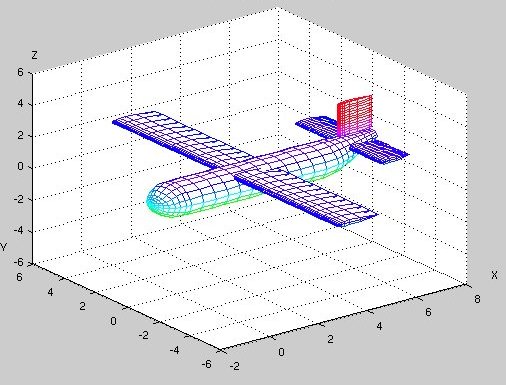 drawn by plane.m
wing_2d.m
rotx_.m
roty_.m
rotz_.m
drawn by plane.m
wing_2d.m
rotx_.m
roty_.m
rotz_.m
OK, long lecture, extra topic:
Generating random numbers, valuable for some testing.
First we generate uniformly distributed random numbers in
the range 0.0 to 1.0. A uniform distribution should have
roughly the same number of values in each range, bin.
Gaussian or Normal distributions should have roughly
a bell shaped curve, based on a given mean and sigma.
Sigma is the standard deviation. Sigma squared is the variance.
udrnrt.h three generators
udrnrt.c three generators code
plot_udrnrt.c test_program
plot_udrnrt1.out udrnrt output and plot
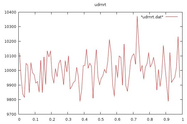 2.0*udrnrt()-1.0 output, -1.0 to 1.0
plot_udrnrt2.out gauss output and plot
2.0*udrnrt()-1.0 output, -1.0 to 1.0
plot_udrnrt2.out gauss output and plot
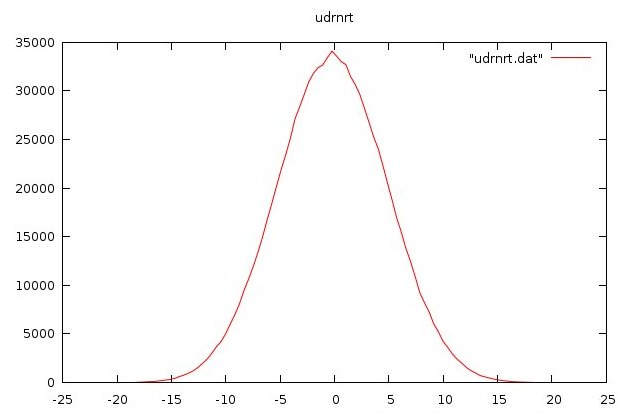 plot_udrnrt3.out gauss output and plot
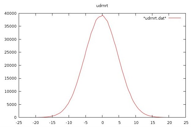 plot_udrnrt4.out sine wave output and plot
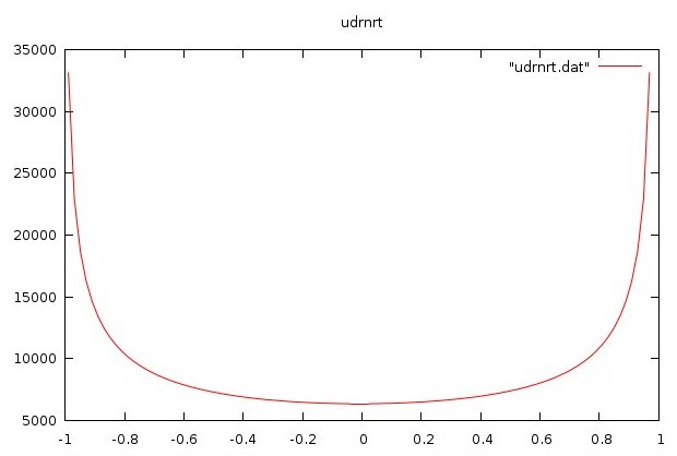 test_rand.py uniform and gauss plot
test_rand.py3 uniform and gauss plot
test_rand.py uniform and gauss plot
test_rand.py3 uniform and gauss plot
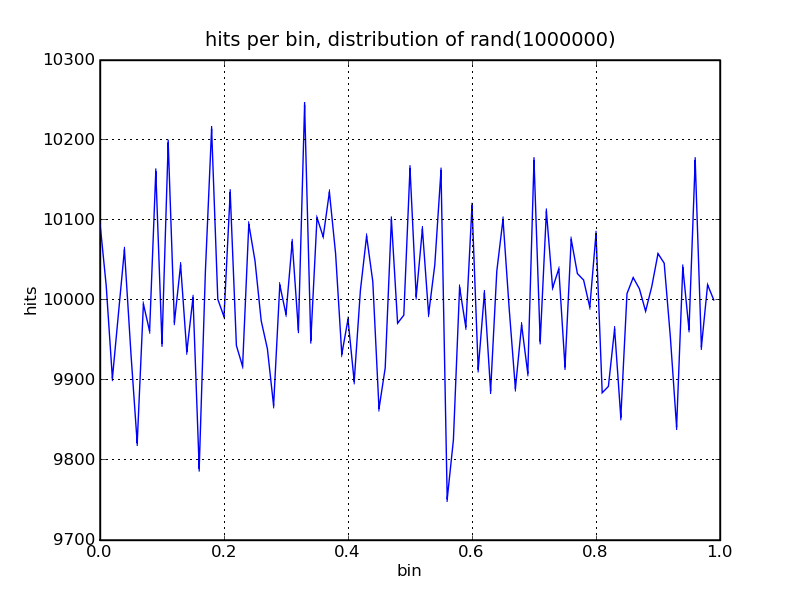 1,000,000 uniformly distributed samples
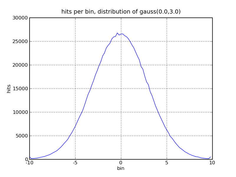 1,000,000 Gaussian distributed samples, mean=0.0, sigma=3.0
HW3 due by midnight of next class
1,000,000 Gaussian distributed samples, mean=0.0, sigma=3.0
HW3 due by midnight of next class
Creating a numerical algorithm can take years.
Finding and adapting a numerical algorithm is practical.

The 10 top programming languages:
most used
2019 chart
learn a programming language

Some history and dates of programming languages:
http://en.wikipedia.org/wiki/History_of_programming_languages

LAPACK is a good starting place to find high quality numerical code.
Yes, much is in Fortran 77, some in Fortran 95, and yes much of the code
is a very mature 30 years old. The good news is that the code produces
correct numeric results with known accuracy. A download typically
includes test drivers and timing programs.

LAPACK is used in Maple, Matlab, and libraries are available for
C, Python, Ruby, Java, Ada, and many other languages.

see www.netlib.org/lapack

ACM Transactions on Mathematical Software, TOMS is another
source. see www.netlib.org/toms

LAPACK includes prior LINPACK and EISPACK and uses the BLAS,
Basic Linear Algebra Subroutines, for low level operations.

Almost every LAPACK routine is available in four types:
  Single precision floating point  prefix "s"
  Double precision floating point  prefix "d"
  Complex single precision         prefix "c"
  Complex double precision         prefix "z"


LAPACK is available on Internet:

LAPACK FAQ
naming conventions
single
double
complex
complex16

LAPACK Users Guide

lapcak.index information

The Fortran source code for the Linear Algebra Package, LAPACK
are under the LAPACK directory with subdirectories
   SRC  BLAS  TESTING  TIMING  INSTALL
On CSEE Help WEB pages:  www.csee.umbc.edu/help/fortran
And, for g95 users, the Fortran95 interface
UMBC CSEE help, then fortran
then BLAS
libblas.a
liblapack.a

Or, on Debian or Ubuntu  sudo apt-get install gfortran
and compile and link LAPACK and all my examples.


lapack.tar big, about 35MB
LAPACK installation guide (postscript)
LAPACK quick reference (PostScript)
Raw LAPACK directory use lapack.a and blas.a on Linux on Intel
Raw LAPACK/SRC directory
Raw LAPACK/BLAS directory
Raw LAPACK/TESTING directory
Raw LAPACK/TIMING directory
Raw LAPACK/INSTALL directory
lapcak95.tgz

g95 for Linux, tar -xvzf g95-x86-linux.tgz
Self installing executable,g95 for MS Windows

Much more information on Fortran, including a full manual, is at
www.csee.umbc.edu/help/fortran


For Java users:
Java Numerics WEB Site
includes an early version of LAPACK translated to Java plus many other
numeric routines.


For Python users: Python has numpy and scipy and can call Fortran code
Python bindings


For Ada users there is an interface binding
Ada bindings


For Scala users: No LAPACK I could find, alternative
Scalala math library


There is a learning curve to using LAPACK.
I suggest finding a routine you need.
Copy the comments from the front of that routine into your program.
Create the necessary declarations needed for calling the routine.
Create a Makefile with the compilation and library commands.
You will need lapack.a and blas.a or equivalent.

An example use on our CSEE system is
Makefile_LAPACK
test_eigen2.f90
test_eigen2_f90.out
This is really old code that still works and uses
invrse.for
eigdet.for
matmul.for
evalvec.for
a02ftext.for
When 64-bit floating point is not accurate enough
When 64-bit integers are way too small

You will need this lecture for Homework 4 and
cs455 Project

"C" has gmp, gnu multiple precision.

Java has a bignum package.
Java has apfloat.jar

Ada has arbitrary decimal digit precision floating point.

Fortran has a multiple precision library.

Python has arbitrary precision integer arithmetic
Python has mpmath and other packages

Hmmm? Multiple precision must be important and have a use.

Computing Pi to a million places is a demonstration, but there
are more reasonable uses.

Types of multiple precision:
  Unlimited length integers
  Unlimited length fractions  1/integer
  Unlimited length rationals  integer/integer
  Unlimited length floating point
  Arbitrary yet fixed number of digits floating point


for "C" get gmp, GNU Multiple Precision!
download gmp from https://gmplib.org
gmp.guide

Here are a few simple gmp samples

test_mpf.c
test_mpf.out
test_mpq.c
test_mpq.out
test_mpz.c
test_mpz.out
gmp fact.c
fact_gmp.out


Java BigDecimal that is BigInteger with a scale factor
Big_pi.java test program
Big_pi_java.out test results
Big_pi_check.java test program
Big_pi_check_java.out test results
test_apfloat.java test program
test_apfloat.out test results
mytest_apfloat.java test program
mytest_apfloat.out test results
Big_math.java various functions exp, sin
Big_simeq.java simultaneous equations
Big_inverse.java invert matrix

Fortran 95 module that implements big integers
big_integers_module.f90
test_big.f90  test program
test_big_f90.out  test results

Ada 95 precise, rational and digits arithmetic
directory of Ada 95 files

Python simple factorial(52) is
factorial.py  program
factorial_py.out  output
factbig.py3  really big 1,000,000!


Python simple 2^200 integer, yet floating point is IEEE 64 bit
power2.py  program
power2_py.out  output
test_mpmath.py  program
test_mpmath_py.out  output
test_mpmath.py3  program
test_mpmath_py3.out  output
mpmath_example.py  program
mpmath_example_py.out  output
mpmath_example.py3  program
mpmath_example_py3.out  output


A quick conversion of simeq.c to mpf_simeq.c solves simultaneous
equations with 50 digits, could be many more digits using gmp mpf_t.

Using the very difficult to get accurate answers matrix:

test_mpf_simeq.c
mpf_simeq.c
mpf_simeq.h
test_mpf_simeq.out
test_mpf_simeq_300.out


Can irrational numbers be combined to produce an integer?

It appears that  e^(Pi*sqrt(163)) is the integer 262,537,412,640,768,744
and that is rather amazing to me.

How might this be validated? It has been tried using higher and
higher precision and the value computes to about
262,537,412,640,768,743.999,999,999,999,999,999,999

We know 1.5 base 10 can be represented as  1.1 base 2 exactly.
We know 1/3 can not be represented exactly in a finite number of
decimal digits or a finite number of binary digits
   1/3 = 0.3333333333333333333333333333333  decimal approximately
   1/3 = 0.0101010101010101010101010101010  binary approximately
And, for what it is worth
We know 1/3 can be represented exactly as  0.1 base 3.

A quick "C" program gives the first 14 digits, using IEEE 64-bit floating point

 /* irrational.c  e^(Pi*sqrt(163)) is an integer?  */
 #include <math.h>
 #include <stdio.h>

 #define e  2.7182818284590452353602874713526624977572
 #define Pi 3.1415926535897932384626433832795028841971

 int main(int argc, char * argv[])
 {
   printf("e^(Pi*sqrt(163)) is an integer? \n");
   printf("  262537412640768744.0000000  check \n");
   printf("%28.7f  using 15 digit arithmetic \n",pow(e,Pi*sqrt(163.0)));
   return 0;
 }
With output:
 e^(Pi*sqrt(163)) is an integer?
   262537412640768744.0000000  check
   262537412640767712.0000000  using 15 digit arithmetic
   262537412640768743.99999999999925007259719818568887935385633733699 using 300 digit

What is needed is to show convergence from above and below,
and it would be nice if the convergence was uniform. This
could use 50, 100, 150, 200 digit precision for the computation.
Pick a number of digits. Increment the bottom digit of e, Pi and 163
then do the computation. Decrement the bottom digit of e, Pi and 163
then do the computation. Check if the upper and lower values of
the fraction are converging toward zero. Check if the convergence
is uniform, balanced, for the upper and lower values.

This is left as an exercise to the student.

Computing Pi to arbitrary precision

One method of computing Pi is to compute 4*atan(1) or
24*atan(b2)  b2=(2*sqrt(b1)-1)/b1  b1=2-sqrt(3)
get_pi.c
get_pi.out
get_pi.c using double and math.h atan
pi=24*atan(b2) b2=0.131652, b1=0.267949
    Pi= 3.1415926535897932384626433832795028841971
get_pi= 3.14159265358980333
 pi-Pi= 0.00000000000001021

get_mpf_pi.c
get_mpf_pi.out
get_mpf_pi.c using digits=50
b1=    0.26794919243112270647255365849412763305719474618962
b2=    0.13165249758739585347152645740971710359281410222324
mpf_pi= 3.1415926535897932384626433832795028841971693999457
    Pi= 3.1415926535897932384626433832795028841971


Now you can do Homework 4


Using gmp to solve higher power methods

For reference in later lectures on PDE, when "double" is
just not accurate enough to allow higher power methods:

Solving a relatively simple partial differential equation

    du/dx + du/dy = 0

using a uniform grid on rectangle 0 <= X <= 2Pi, 0 <= Y <= 2Pi
with boundary values (and analytic solution)

    u(x,y) = sin(x-y)

Due to the symmetry of the problem, the number of boundary
points in X and Y can not be the same. If nx = ny then
the solution of simultaneous equations becomes unsolvable
because of a singular matrix.

Solutions above nx or ny equal 13 cause unstable values
for the derivative coefficients with standard nderiv
computation. Actually, integer overflow occurs first.

By using gmp with high precision integer, mpz, and
high precision floating point, mpf, then high
accuracy solutions can be computed.

Setting "digits" at 200, "bits" becomes 200*3.32 = 664.
This is used for computing boundary values and the
numeric checking against the analytic solution.

The results are:
  nx  ny  maxerror
  13  12  1.40e-4     same as nx=12, ny=13, they can not be equal
  15  14  4.38e-6
  17  16  1.02e-7
  19  18  1.84e-9
  21  20  2.70e-11
  23  22  3.23e-13
  25  24  3.23e-15
  31  30  1.25e-21
  33  32  6.86e-24
  35  34  3.33e-26
  37  36  1.44e-28

  37  36  8.59e-18  0  to  4Pi
  37  36  3.40e-7   0  to  8Pi

The basic "C" code with lots of printout is:
source code pde2sin_eq.c
output pde2sin_eq_c.out
source code pde2sin_sparse.c
output pde2sin_sparse_c.out

The same programs, converting "double" to gmp "mpf_t"
and calling gmp versions of functions is:
source code pde2sin_eq_gmp.c
output pde2sin_eq_gmp.out
source code pde2sin_sparse_gmp.c
output pde2sin_sparse_gmp.out
gmp function mpf_deriv.h
gmp function mpf_deriv.c
gmp function mpf_simeq.h
gmp function mpf_simeq.c
gmp function mpf_sparse.h
gmp function mpf_sparse.c

Then, using non uniform derivative (on same uniform grid):
source code pde2sin_nueq_gmp.c
output pde2sin_nueq_gmp.out
source code pde2sin8_nueq_gmp.c
output pde2sin8_nueq_gmp.out
source code pde4sin_nueqsp.c
output pde4sin_nueqsp.out
gmp function mpf_nuderiv.h
gmp function mpf_nuderiv.c
gmp function mpf_inverse.h
gmp function mpf_inverse.c
gmp function mpf_simeq.h
gmp function mpf_simeq.c
gmp function mpf_sparse.h
gmp function mpf_sparse.c

binary.txt convert binary to decimal

multiple precision HW4 is assigned
Finding Roots

First, a special case, the "roots of unity"
 x  +1=0  root is x=-1
 x^2+1=0  roots are x=i  x=-i  i=sqrt(-1)
 x^3+1=0  roots are x=-1 x=1/2 +i sqrt(3)/2 x=1/2 -i sqrt(3)/2
 x^4+1=0  roots are x=+sqrt(2)/2 +i sqrt(2)/2
                      (all four combinations of +/-)

 Note that all roots are on the unit circle in the complex plane.

Consider the Maple root finding for x^12+1=0 :

root12g.html

In general the roots of a polynomial are complex numbers.
A general purpose root finder for polynomials is difficult to
develop. Fortunately, some very smart people have written the
function, cpoly, that can take a general polynomial with complex
coefficients and find the complex roots. It also works with
real coefficients and real roots.

MatLab root finding for polynomials is just r = roots(p)
Where p is the vector of polynomial coefficients and
r is the vector of roots. Both r and p may be complex.
find_roots.m source code
find_roots_m.out output

Maple root finding for polynomials, not great:
find_roots.mws source code
find_roots_mws.out output
real and complex work some times.

Finding roots of a polynomial seems easy:

  given  c_n x^n + c_n-1 x^n-1 + ... _ c_1 x + c_0 = 0

  find a value, x=r, that satisfies the equation,
  divide the polynomial by  (x-r) and thus have a
  polynomial of one degree lower. Repeat. Done.

  Unfortunately there are a lot of pitfalls, solved by the codes below.
  Standard techniques include dividing through by c_n,
  if c_0 is zero, there is a root equal zero, divide through by x,
  if highest power is 2, directly solve the quadratic equation.

"cpoly" is a very old routine to compute roots of a polynomial
with complex coefficients c_0 ... c_n.

The Fortran code, including the test program (driver) for  cpoly  is
419.for in Fortran IV, compiles with g95
419_f.out is the output of many test cases

Another version, with an automatic conversion of Fortran to C.
The program  f2c  converts .f to .c  it may not be very pretty.
It also needs the library that comes with  f2c.
419.f driver and cpoly
419.c driver and cpoly


The Java code, including the test program (driver) is
c419.java in standard Java
c419.out is the output of many test cases

The Ada code, including the test program (driver) is
long_complex_polynomial_roots.ada in Ada


To understand how some iterative methods can converge quickly,
consider how to compute sqrt when you have no math library:
  Basically y=sqrt(x)  guess y, y_next = (x/y+y)/2, repeat.
    Do not guess zero for y, x/y does not work, use y = 1 as guess.


sqrt.c
sqrt_c.out

A professional implementation of sqrt would reduce the input, x,
to a range from 0.25 to 1.0 by dividing by an even power of 2.
The sqrt(x^2n) is just x^n. The square root of a product is
the product of the square root of the factors. This can be easy
with IEEE floating point numbers because they are stored with
an exponent of 2.


So, since the sqrt iteration was basically Newtons method,
why not just use Newtons method to find roots?
here is how it works, even for complex roots.

Given: f(x) = 0
guess x
x_next = x - f(x)/f'(x)   f'(x) is the derivative of f(x)
                          avoid region where slope is zero
repeat until |x_next-x| < epsilon

newton.c
newton_c.out

Notice the oscillation in the last few steps.
The problem can come from a bad guess that causes a big
oscillation. The problem can come from hitting an x
where f'(x) is zero. Thus, there have been many workarounds.
"cpoly" is one of the most general solutions.

Nonlinear Equations

Other examples:
given  f(x) = x + 2 x^2 + 3/x = 6
thus   f'(x) = 1 + 4 x - 6/x^2
then  guess a value of x,  Newton iteration is
next  x = x - f(x)/f'(x)

First, expect x=1,  we happen to have at least two possible solutions:
simple_nl.c
simple_nl_c.out

Second, expect x=2, have convergence to expected solution:
simple2_nl.c
simple2_nl_c.out

Systems of Nonlinear Equations
in matrix form, the equations are: A * X = Y
| 1  2  3 |   |  x1  | = | 10.000 |
| 2  1  1 | * | x2^2 | = |  6.333 |
| 3  1  4 |   | 1/x3 | = |  8.333 |
     A      *    X     =     Y

from equations that have these derivatives
 f1(x1, x2, x3) = x1 + 2 x2^2 + 3/x3 = 10
 f1'(x1) = 1
 f1'(x2) = 4 x2
 f1'(x3) = -3/x3^2

 f2(x1, x2, x3) = 2 x1 + x2^2 + 1/x3 = 6.333
 f2'(x1) = 2
 f2'(x2) = 2 x2
 f2'(x3) = -1/x3^2

 f3(x1, x2, x3) = 3 x1 + x2^2 + 4/x3 = 8.333
 f3'(x1) = 3
 f3'(x2) = 2 x2
 f3'(x3) = -4/x3^2

create the Jacobian
     |   1    |   | 1   4*x2  -3/x3^2 |
 A * | 2*x2   | = | 2   2*x2  -1/x3^2 | = Ja
     |-1/x3^2 |   | 3   2*x2  -4/x3^2 |
 A *     D      =        Ja
     deriv of X   wrt x1,x2,x3

The Newton iteration becomes
 next X = X - (A*X-Y)/Ja,  /Ja is times transpose inverse of Ja
 Ja is, in general, dependent on all variables

Three equations in three unknowns, not direct convergence.
Experiments show great difference with widely different
initial conditions. Two sets of equations with a choice of
initial condition. x1, x2, x3 are the variables.
equation_nl.c
equation_nl_c.out
inverse.c used by code above

In other languages:
equation_nl.adb
equation_nl_ada.out
inverse.adb
equation_nl.f90
equation_nl_f90.out
inverse.f90
equation_nl.java
equation_nl_java.out
inverse.java


A system of non linear equations with powers 1, 2, 3, -1 and -2.
This example has a lot of debug print and several checks.
Added is also, variable control of fctr, a multiplier on
how much correction is to be made each iteration.
The problem and method are described as comments in the code.
equation2_nl.adb
equation2_nl_ada.out

Same example as above, in various languages, with debug removed:
equation2_nl.f90
equation2_nl_f90.out
equation2_nl.c
equation2_nl_c.out
equation2_nl.java
equation2_nl_java.out

A polynomial nonlinear example that converges with no fctr control.
equation4_nl.c
equation4_nl_c.out

A more general routine for solving a system of nonlinear
simultaneous equations A x = y where there are n unknowns and
any unknown may be first, second, third power of negative one
or negative two power:
A is n by n+nonlinear terms.
y is n right hand sides of equations
x is n+nonlinear, initially the first guess at solution
of the linear terms with space for non linear terms.

The caller sets up var1 with indices of first power.
The caller sets up var2 with indices of second power.
The caller sets up var3 with indices of third power.
The caller sets up vari1 with indices of negative first power.
The caller sets up vari2 with indices of negative second power.
Must have each term, then non linear, note: -1 means no term

a*x[0] + b*x[0]*x[1]*x[2] + c*x[1]*x[1]*x1[1]/(x[0]*x[2]) = d
n=3 variables, nonlinear=2 in this example

              x[0] x[1] x[2]   b    c
int var1[]  = { 0,   1,   2,   0,   1 }; // zero based subscript
int var2[]  = {-1,  -1,  -1,   1,   1 }; // e.g. last is x3*x4
int var3[]  = {-1,  -1,  -1,   2,   1 }; // possible cube or 3 term
int vari1[] = {-1,  -1,  -1,  -1,   0 }; // zero based subscript
int vari2[] = {-1,  -1,  -1,  -1,   2 }; // e.g. last is x3*x4

simeq_newton5.java
test_simeq_newton5.java
test_simeq_newton5_java.out
inverse.java

simeq_newton5.py3
test_simeq_newton5.py3
test_simeq_newton5_py3.out
A difficult numerical problem is the finding of a global minima
of an unknown function. This type of problem is called an
optimization problem because the global minima is typically
the optimum solution.
In general we are given a numerically computable function of
some number of parameters v = f(x_1, x_2, ... , x_n)
and must find the values of x_1, x_2, ... , x_n that gives
the smallest value of v. Or, by taking the absolute value,
find the values of x_1, x_2, ... , x_n that give the value
of v closest to zero.
Generally the problem is bounded and there are given maximum and
minimum values for each parameter. There are typically many
places where local minima exists. Thus, the general solution
must include a global search then a local search to find the
local minima. There is no general guaranteed optimal solution.
First consider a case of only one variable on a non differentiable
function, y = f(x) where x has bounds xmin and xmax. There may be
many local minima, valleys that are not the deepest.
* * * * *
* * * * * * * * * *
* * * * * * * * * * *
* * * ** * * *
* *
*
Global search:
Do a y=f(x) for x = xmin, x = x+dx, until x>xmax,
Save the smallest y and the x0=x for that y.
Then find the local minimum:
Consider evaluating f(x) at some initial point x0 and x0+dx.
If f(x0) < f(x0+dx) you might move to x0-dx.
if f(x0) > f(x0+dx) you might move to x0+dx+dx.
The above may be very bad choices!
Here are the cases you should consider:
Compute yl=f(x-dx) y=f(x) yh=f(x+dx) for some dx
yh y yh y yl yl
y yh yl yl yh y
yl yl y yh y yh
case 1 case 2 case 3 case 4 case 5 case6
For your next three points, always keep best x:
case 1 x=x-dx possibly dx=2*dx
case 2 x=x-dx dx=dx/2
case 3 dx=dx/2
case 4 x=x+dx dx=dx/2
case 5 dx=dx/2
case 6 x=x+dx possibly dx=2*dx
Then loop.
A simple version in Python is
optm.py
optm_py.out
optm.py running
minimum (x-5)**4 in -10 to +10 initial 2, 0.001, 0.001, 200
xbest= 5.007 , fval= 2.401e-09 ,cnt= 21
minimum (x-5)**4 in -10 to +10 initial 2 using default
xbest= 4.998271 , fval= 8.9367574925e-12 ,cnt= 35
Another version, found on the web, slightly modified
min_search.py
min_search_py.out
min of (x-5)**4, h= 0.1
xmin= 4.9984375
fmin= 5.96046447754e-12
n= 86 , sx= 4.996875 , xx= 5.003125
min of (x-5)**4, h= 0.01 # smaller initial h, not as good
xmin= 4.9975
fmin= 3.90625000037e-11
n= 704 , sx= 4.995 , xx= 5.005
min of (x-5)**4, h= 2.0 # smaller tolerance, better
xmin= 4.99993896484
fmin= 1.38777878078e-17
n= 47 , sx= 4.99987792969 , xx= 5.00012207031
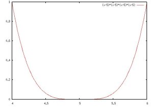
Beware local minima
Both of the above, will find the best of a local minima.
There could be a local minima, thus when dx gets small enough,
remember the best x and use another global search value to
look for a better optimum. Some heuristics may be needed to
increase dx. This is one of many possible algorithms.
Another algorithm that is useful for large areas in two
dimensions for z=f(x,y) is:
Use a small dx and dy to evaluate a preferred direction.
Use an expanding search, doubling dx and dy until no more
progress is made. Then use a contracting search, halving dx and dy
to find the local minima on that direction.
Repeat until the dx and dy are small enough.
The numbers indicate a possible order of evaluation of the points
(in one dimension).
1
2
3
5
6
7 Value computed
4 ^
8 |
9
------------> X direction
Numbers are sample number.
Note dx doubles for samples 2, 3, 4, 5
then dx is halved and added to best so far, 4, to get 6
then halved to get 7, 8, 9.
There may be many expansions and contractions.
The pseudo derivatives are used to find the preferred direction:
(After finding the best case from above, make positive dx and dy best.)
z=f(x,y)
zx=f(x+dx,y) zx < z
zy=f(x,y+dy) zy < z
r=sqrt(((z-zx)^2+(z-zy)^2))
dx=dx*(z-zx)/r
dy=dy*(z-zy)/r
This method has worked well on the spiral trough.
The really tough problems have many discontinuities.
I demonstrated a function that was everywhere discontinuous.
The function was f(x)=x^2-1 with f(x)=1 if the bottom bit
of x^2-1 is a one.
discontinuous.c first function
discontinuous.out
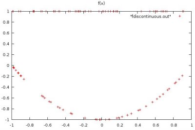 Another, recursive, function that is continuous, yet in the
limit of recursing, nowhere differentiable, is:
double f(x){ /* needs a termination condition, e.g count=40 */
if(x<=1.0/3.0) return (3.0/4.0)*f(3.0*x);
else if(x>=2.0/3.0) return (1.0/4.0)+(3.0/4.0)*f(3.0*x-2.0);
else /* 1/3 < x < 2/3 */
return (1.0/4.0)+(1.0/2.0)*f(2.0-3.0*x);}
discontinuous.c second function
discontinuous.out
Another, recursive, function that is continuous, yet in the
limit of recursing, nowhere differentiable, is:
double f(x){ /* needs a termination condition, e.g count=40 */
if(x<=1.0/3.0) return (3.0/4.0)*f(3.0*x);
else if(x>=2.0/3.0) return (1.0/4.0)+(3.0/4.0)*f(3.0*x-2.0);
else /* 1/3 < x < 2/3 */
return (1.0/4.0)+(1.0/2.0)*f(2.0-3.0*x);}
discontinuous.c second function
discontinuous.out
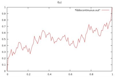 In general, it will not work to use derivatives, or even pseudo
derivatives without additional heuristics.
A sample program that works for some functions of three
floating point parameters is shown below. Then, a more general
program with a variable number of parameters is presented
with a companion crude global search program.
Two parameter optimization in Python useful for project
optm2.py3 source code
optm2_py3.out output
global_search.py3 source code
search_py3.out output
search.py3 source code
search2_py3.out output
notice that zbest stops getting better at some small dx, dy
mpmath_example.py3 source code
mpmath_example_py3.out output
test_mpmath.py3 source code
test_mpmath_py3.out output
Two parameter optimization in java
global_search.java source code
global_search_java.out output
search2.java source code
search2_java.out output
notice that zbest stops getting better at some small dx, dy
Three parameter optimization:
optm3.h
optm3.c
test_optm3.c
test_optm3_c.out
N parameter optimization in C and java:
This includes a global search routine srchn.
optmn.h
optmn.c
test_optmn.c
test_optmn_c.out
optmn_dev.java
test_optmn_dev.java
test_optmn_dev_java.out
optmn_interface.java
optmn_function.java user modifies
optmn.java
optmn_run.java
optmn_run_java.out
In MatLab use "fminsearch" see the help file.
Each search is from one staring point.
You need nested loops to try many starting points.
I got error warnings that I ignored, OK to leave them in your output.
optm.m
An interesting test case is a spiral trough:
In general, it will not work to use derivatives, or even pseudo
derivatives without additional heuristics.
A sample program that works for some functions of three
floating point parameters is shown below. Then, a more general
program with a variable number of parameters is presented
with a companion crude global search program.
Two parameter optimization in Python useful for project
optm2.py3 source code
optm2_py3.out output
global_search.py3 source code
search_py3.out output
search.py3 source code
search2_py3.out output
notice that zbest stops getting better at some small dx, dy
mpmath_example.py3 source code
mpmath_example_py3.out output
test_mpmath.py3 source code
test_mpmath_py3.out output
Two parameter optimization in java
global_search.java source code
global_search_java.out output
search2.java source code
search2_java.out output
notice that zbest stops getting better at some small dx, dy
Three parameter optimization:
optm3.h
optm3.c
test_optm3.c
test_optm3_c.out
N parameter optimization in C and java:
This includes a global search routine srchn.
optmn.h
optmn.c
test_optmn.c
test_optmn_c.out
optmn_dev.java
test_optmn_dev.java
test_optmn_dev_java.out
optmn_interface.java
optmn_function.java user modifies
optmn.java
optmn_run.java
optmn_run_java.out
In MatLab use "fminsearch" see the help file.
Each search is from one staring point.
You need nested loops to try many starting points.
I got error warnings that I ignored, OK to leave them in your output.
optm.m
An interesting test case is a spiral trough:
 Possibly a better view:
 test_spiral.f90
test_spiral_f90.out
spiral.f90
test_spiral.c
test_spiral_c.out
spiral.h
spiral.c
test_spiral.java
test_spiral_java.out
test_spiral.f90
test_spiral_f90.out
spiral.f90
test_spiral.c
test_spiral_c.out
spiral.h
spiral.c
test_spiral.java
test_spiral_java.out
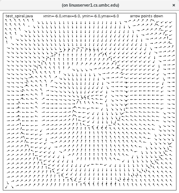 spiral_trough.py
test_spiral.py
test_spiral_py.out
Your project is a multiple precision minimization
See Lecture 15 for multiple precision
spiral_trough.py
test_spiral.py
test_spiral_py.out
Your project is a multiple precision minimization
See Lecture 15 for multiple precision
Sound, voice, music, etc. can be in many compressed formats in
many file types, such as .wav .mp3 .aac .avi .mka .mpeg .vox ...
If your computer has a speaker and software, you can hear sound files.
On almost all browsers, click and hear sound files.
On Ubuntu programs aplay, Rythmbox, and some languages provide
for listening to sound files. There are a few programs that can be
downloaded that convert some type of sound file to another type
of sound file. 30,000 volume samples per second is common.
sudo apt install aplay
We will read a sound file, volume data at very small
time intervals, use FFT to get frequency domain.
Modify the frequency domain, IFFT to get volume and convert
to a .wav file.
A basic Fourier transform can convert a function in the time domain
to a function in the frequency domain. For example, consider a sound
wave where the amplitude is varying with time. We can use a discrete
Fourier transform on the sound wave and get the frequency spectrum.
This is short_count.wav one, two, three
short_count.wav
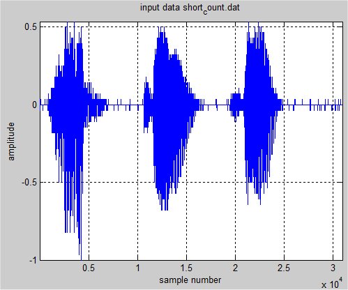 The basic FFT plotting the magnitude of about 31,000 bins
has zero frequency on left, highest frequency in middle,
and back to lowest frequency on right:
The basic FFT plotting the magnitude of about 31,000 bins
has zero frequency on left, highest frequency in middle,
and back to lowest frequency on right:
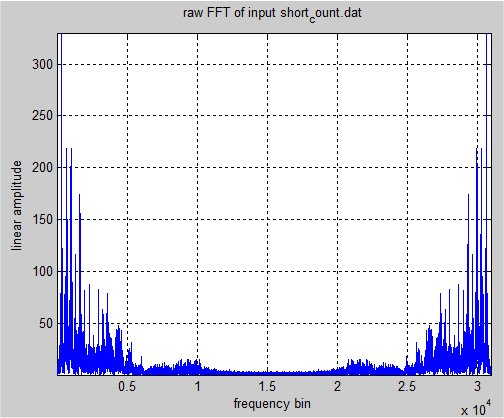 Using fftshift to center the zero frequency:
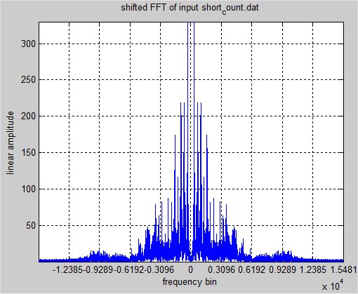 Then taking the log of the amplitude is typical
when plotting a spectrum:
Then taking the log of the amplitude is typical
when plotting a spectrum:
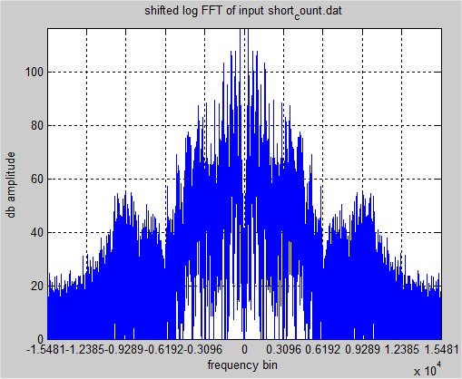 Above made using:
plot_fft.m reads .dat amplitudes
wav_to_dat.c make .dat from .wav
cat.wav, sound file, was converted cat.dat, amplitude data file
cat.wav sound
cat.dat amplitude in 18,814 time steps
Of course there is an inverse Fourier transform that converts
the frequency spectrum back to the time domain.
The spectrum of F(t)=sin(2 Pi f t) t=0..1 is a single frequency f.
The discrete transform assumes the function is repeated for all t.
The amplitude values must be sampled at equal time increments for
the spectrum to be valid. The maximum frequency that can be
computed, called the Nyquist Frequency, is one half the sampling rate.
Sampling at 10,000 samples per second has maximum frequency of 5kHz.
It turns out that a signal at some frequency has an amplitude and
a phase, or an in-phase and quadrature value. The convenient
implementation is to consider these values as complex numbers.
It turns out that some input can be collected as complex values and
thus most implementations of the FFT take an array of complex numbers
as input and produce the same size array of complex numbers as output.
For technical reasons, a simple FFT requires the size of the input
and output must be a power of 2. Special versions of the FFT as found in
FFTW the fastest Fourier transform in the west
handle arbitrary sizes. We just pad out our input data with zeros to make
the size of the array a power of 2.
Fourier transforms have many other uses such as image filtering and
pattern matching, convolution and understanding modulation.
A few, non fast, programs that compute Fourier Series coefficients for
unequally spaced samples, read from a file, are:
fourier.c
fourier.java
sin(2x) data sin2.dat
test on sine2.dat fourier_java.out
More detail of the basic Fourier transforms and series,
both continuous and discrete is fourier.pdf
square_wave_gen.c using series
square_wave_gen_c.out cos and sin
There are many many implementations of the FFT, the n log_2 n
complexity method of computing the discrete Fourier transform.
Two of the many methods are shown below.
One method has the coefficients precomputed in the source code.
A second method computes the coefficients as they are needed.
Precomputed constants for each size FFT
fft16.c fft16.adb
fft32.c fft32.adb
fft64.c fft64.adb
fft128.c fft128.adb
fft256.c fft256.adb
fft512.c fft512.adb
fft1024.c fft1024.adb
fft2048.c fft2048.adb
fft4096.c fft4096.adb
Precomputed constants of each size inverse FFT
ifft16.c ifft16.adb
ifft32.c ifft32.adb
ifft64.c ifft64.adb
ifft128.c ifft128.adb
ifft256.c ifft256.adb
ifft512.c ifft512.adb
ifft1024.c ifft1024.adb
ifft2048.c ifft2048.adb
ifft4096.c ifft4096.adb
Header file and timing program
fftc.h
fft_time.c fft_time.adb
fft_time_c.out fft_time_ada.out
A more general program that can compute the fft and inverse fft for
an n that is a power of two is:
fft.h
fft.c
fftest.c
fftin.dat binary data
fftin.out binary data
A more general program for the FFT of large data in Java is:
Cxfft.java
read_wav.java reads and writes .wav
read_wave_java.out output
these may be combined for use in HW5.
fft_wav.java transform and inverse
fft_frame.java with a very crude frequency plot
Above made using:
plot_fft.m reads .dat amplitudes
wav_to_dat.c make .dat from .wav
cat.wav, sound file, was converted cat.dat, amplitude data file
cat.wav sound
cat.dat amplitude in 18,814 time steps
Of course there is an inverse Fourier transform that converts
the frequency spectrum back to the time domain.
The spectrum of F(t)=sin(2 Pi f t) t=0..1 is a single frequency f.
The discrete transform assumes the function is repeated for all t.
The amplitude values must be sampled at equal time increments for
the spectrum to be valid. The maximum frequency that can be
computed, called the Nyquist Frequency, is one half the sampling rate.
Sampling at 10,000 samples per second has maximum frequency of 5kHz.
It turns out that a signal at some frequency has an amplitude and
a phase, or an in-phase and quadrature value. The convenient
implementation is to consider these values as complex numbers.
It turns out that some input can be collected as complex values and
thus most implementations of the FFT take an array of complex numbers
as input and produce the same size array of complex numbers as output.
For technical reasons, a simple FFT requires the size of the input
and output must be a power of 2. Special versions of the FFT as found in
FFTW the fastest Fourier transform in the west
handle arbitrary sizes. We just pad out our input data with zeros to make
the size of the array a power of 2.
Fourier transforms have many other uses such as image filtering and
pattern matching, convolution and understanding modulation.
A few, non fast, programs that compute Fourier Series coefficients for
unequally spaced samples, read from a file, are:
fourier.c
fourier.java
sin(2x) data sin2.dat
test on sine2.dat fourier_java.out
More detail of the basic Fourier transforms and series,
both continuous and discrete is fourier.pdf
square_wave_gen.c using series
square_wave_gen_c.out cos and sin
There are many many implementations of the FFT, the n log_2 n
complexity method of computing the discrete Fourier transform.
Two of the many methods are shown below.
One method has the coefficients precomputed in the source code.
A second method computes the coefficients as they are needed.
Precomputed constants for each size FFT
fft16.c fft16.adb
fft32.c fft32.adb
fft64.c fft64.adb
fft128.c fft128.adb
fft256.c fft256.adb
fft512.c fft512.adb
fft1024.c fft1024.adb
fft2048.c fft2048.adb
fft4096.c fft4096.adb
Precomputed constants of each size inverse FFT
ifft16.c ifft16.adb
ifft32.c ifft32.adb
ifft64.c ifft64.adb
ifft128.c ifft128.adb
ifft256.c ifft256.adb
ifft512.c ifft512.adb
ifft1024.c ifft1024.adb
ifft2048.c ifft2048.adb
ifft4096.c ifft4096.adb
Header file and timing program
fftc.h
fft_time.c fft_time.adb
fft_time_c.out fft_time_ada.out
A more general program that can compute the fft and inverse fft for
an n that is a power of two is:
fft.h
fft.c
fftest.c
fftin.dat binary data
fftin.out binary data
A more general program for the FFT of large data in Java is:
Cxfft.java
read_wav.java reads and writes .wav
read_wave_java.out output
these may be combined for use in HW5.
fft_wav.java transform and inverse
fft_frame.java with a very crude frequency plot
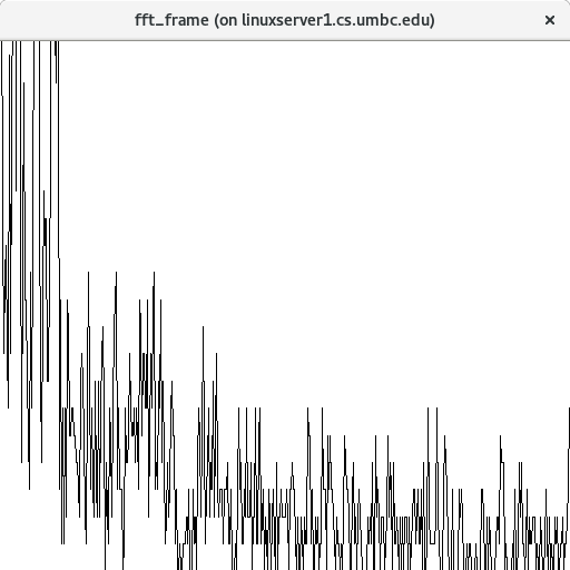 very crude frequency plot
For Matlab, fft_wav.m may be useful for HW5
fft_wav.m transform and inverse, frequency plot
Another version in "C" and Java, the Java demonstrates convolution
fftd.h
fftd.c
test_fft.c
test_fft_c.out
Cxfft.java
TestCxfft.java
TestCxfft.out
Python using downloaded numpy has fft
testfft.py
testfft.out
fftwav.py3
fftwav.py3_out
write_ran_wav.py3
plotwav.py3
print_afile.py3
MatLab has fft as well as almost every other function
test_fft.m
test_fft_m.out
test_fft2.m
test_fft2_m.out
In order to get better accuracy on predicted coefficients
for square wave, triangle wave and saw tooth wave, 1024 points.
The series are shown as comments in the code.
Also shown, is the anti aliasing and normalization needed to
get the coefficients for the Fourier series.
test_fft_big.c
test_fft_big_c.out
very crude frequency plot
For Matlab, fft_wav.m may be useful for HW5
fft_wav.m transform and inverse, frequency plot
Another version in "C" and Java, the Java demonstrates convolution
fftd.h
fftd.c
test_fft.c
test_fft_c.out
Cxfft.java
TestCxfft.java
TestCxfft.out
Python using downloaded numpy has fft
testfft.py
testfft.out
fftwav.py3
fftwav.py3_out
write_ran_wav.py3
plotwav.py3
print_afile.py3
MatLab has fft as well as almost every other function
test_fft.m
test_fft_m.out
test_fft2.m
test_fft2_m.out
In order to get better accuracy on predicted coefficients
for square wave, triangle wave and saw tooth wave, 1024 points.
The series are shown as comments in the code.
Also shown, is the anti aliasing and normalization needed to
get the coefficients for the Fourier series.
test_fft_big.c
test_fft_big_c.out
Reading and Writing .wav files for HW5
Here is a program that just reads a .wav file and writes a copy,
and does a little printing. This with extensions can be the basis
of Homework 5. fftwav.py3 , fft1_wav.c , You may modify
to suit your desires. These only work for single channel, 8 bit
per sample PCM .wav files. (not all the .wav files listed below)
Note: sound does not work from a remote computer, e.g. ssh
Some programs require special libraries or operating systems.
read_wav.c
read_wav.out
train1.wav
short_count.wav
rocky4.wav
cat.wav
Splitting out read and write wav:
rw_wav.h
rw_wav.c
test_rw_wav.c
test_rw_wav.out
And here are three .wav files from very small to larger for testing:
ok.wav
train.wav
roll.wav
fft1t.wav
short_count.wav
fft1c.wav
Suppose you wanted to compute a sound. Here is a generator for
a simple sine wave. It sounds cruddy.
sine_wav.c
sine_wav.out
sine.wav
Computing FFT of a .wav file for HW5
For the homework, one example using a 64 point FFT and just doing
the transform and inverse transform, essentially no change, is
fft1_wav.c
fft1_wav.out
trainf.wav
rockey2.wav
count_out.wav
trainf2.wav experiment
Hopefully you can find some more interesting .wav files.
P.S. When using MediaPlayer or QuickTime be sure to close the
file before trying to rewrite it.
Your web browser can usually play .wav files.
Use file:/// path to your directory /xxx.wav
In Java, ClipPlayer.java reads and
plays .wav and other files. The driver program is ClipPlayerTest.java
In Python, M$ only, with the WX graphics available, play .wav files with
sound.py
or on linux
linux_sound.py
rocky4.wav
In MatLab play .wav, old wave replaced by audio,
must be on local computer with speaker.
waveplay.m
short_count.wav
Im MatLab play .dat files that have a value for each
sample.
soundplay.m
short_count.dat
For students running Ubuntu, this sequence of "C" programs
demonstrate direct use of playing sampled amplitude sound.
These do not require generating a .wav or other type sound file.
pcm_min.c
pcm_sin.c
pcm_dat.c
Makefile_sound
short_count.dat
long_count.dat
You may modify any of these to suit your needs.
An interactive WEB site with with a few functions and their spectrum is
heliso.tripod.com/java_hls/gccs/spectrum1.htm
Here is Rocky speaking and the dynamic spectrum
rocky4.wav
This needs modifications for 2 channel and 16 bits per sample.
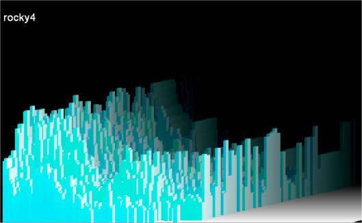 Now you can do homework 5
You may not have your own web page activated to play your .wav files:
do these commands:
cp my.vav ~/pub/www/
cd ~/pub/www/
chmod go+rx my.wav
cd ..
chmod go+rx www
cd ~
you are back in your login directory, and from home you can
http://www.gl.umbc.edu/~your-user-id
then click on my.wav
optional plots of FFT's using Python and C with gnuplot
plot_fft_py.html
plot_fft_c.html
Now sound in db:
cs455_l18a.html
Then FFT to determine material, molecules.
Making spectrum to get wave shape, Gibb to square wave
wave = sum (1.0/g)*sin(g*x) g = 1, 3, 5, 7, 9, ... 75
plot_gibb.py3 source code
plot_gibb_py3.out output
Plotted results:
Now you can do homework 5
You may not have your own web page activated to play your .wav files:
do these commands:
cp my.vav ~/pub/www/
cd ~/pub/www/
chmod go+rx my.wav
cd ..
chmod go+rx www
cd ~
you are back in your login directory, and from home you can
http://www.gl.umbc.edu/~your-user-id
then click on my.wav
optional plots of FFT's using Python and C with gnuplot
plot_fft_py.html
plot_fft_c.html
Now sound in db:
cs455_l18a.html
Then FFT to determine material, molecules.
Making spectrum to get wave shape, Gibb to square wave
wave = sum (1.0/g)*sin(g*x) g = 1, 3, 5, 7, 9, ... 75
plot_gibb.py3 source code
plot_gibb_py3.out output
Plotted results:
 plot_gibb_1.png
 plot_gibb_3.png
 plot_gibb_5.png
 plot_gibb_25.png
 plot_gibb_75.png
Digital Filtering uses numerical computation rather than analog
components such as resistors, capacitors and inductors to
filter out frequency bands.
A low-pass filter will have a "cutoff frequency" f such that
frequencies above f will be attenuated and frequencies below f
will be passed. The filter does not produce a sharp dividing
line and all frequencies are changed in both amplitude and
phase angle.
A high-pass filter will have a "cutoff frequency" f such that
frequencies below f will be attenuated and frequencies above f
will be passed. The filter does not produce a sharp dividing
line and all frequencies are changed in both amplitude and
phase angle.
A band-pass filter will pass frequencies between f1 and f2,
attenuating frequencies below f1 and attenuating frequencies
above f2. f1 <= f2.
The signal v(t)=sin(2 Pi f t) t=t0, t1, ..tn is a single frequency f.
For digital filtering we assume the digital value of v(ti) is
sampled at uniformly spaced times t0, t1,..., tn.
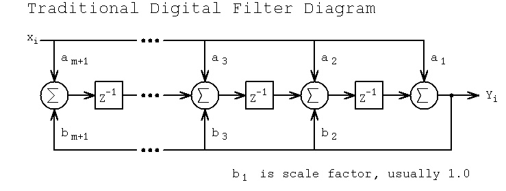 For an order m filter, with one based subscripts:
y(i) = ( a(1)*x(i) + a(2)*x(i-1) + a(3)*x(i-2) + ... + a(m+1)*x(i-m)
- b(2)*y(i-1) - b(3)*y(i-2) - ... - b(m+1)*y(i-m) )/b(1)
For an order m filter, with one based subscripts:
y(i) = ( a(1)*x(i) + a(2)*x(i-1) + a(3)*x(i-2) + ... + a(m+1)*x(i-m)
- b(2)*y(i-1) - b(3)*y(i-2) - ... - b(m+1)*y(i-m) )/b(1)
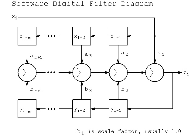 With array x and y in memory, the MatLab code for computing y(1:n) could be:
for i=1:n
y(i)=a(1)*x(i);
for j=1:m
if j>=i
break
end
y(i)=y(i) + a(j+1)*x(i-j) - b(j+1)*y(i-j);
end
y(i)=y(i)/b(1); % not needed if b(1) equals 1.0
end
or, use MatLab y = filter(a, b, x); % less typing
For an order m filter, with zero based subscripts:
y[i] = ( a[0]*x(i) + a[1]*x[i-1] + a[2]*x[i-2] + ... + a[m]*x[i-m]
- b[1]*y[i-1] - b[2]*y[i-2] + ... - b[m]*y[i-m] )/b[0]
With array x and y in memory, the C code for computing y[0] to y[n-1] could be:
for(i=0; i<n; i++) {
y[i]=a[0]*x[i];
for(j=1; j<=m; j++)
{
if(j>i) break;
y[i]=y[i] + a[j]*x[i-j] - b[j]*y[i-j];
}
y[i]=y[i]/b[0]; /* not needed if b[0]==1 */
}
For reading x samples and writing filtered y values:
read next x sample and compute y and output y
(the oldest x and y in RAM are deleted and the new x and y saved.
Typically use a circular buffer [ring buffer] so that the saved x and y
values do not have to be moved [many uses of modulo in this code].)
Given a periodic input, filters require a number of samples to build up
to a steady state value. There will be amplitude change and phase change.
Typical symbol definitions related to digital filters include:
ω = 2 Π f
z = ej ω t digital frequency
s = j ω analog frequency
z-1 is a unit delay (previous sample)
IIR Infinite Impulse Response filter or just recursive filter.
In transfer function form
yi a0 + a1 z-1 + a2 z-2 + a3 z-3 + ...
---- = -----------------------------------
xi b1 z-1 + b2 z-2 + b3 z-3 + ...
s = c (1-z-1)/(1+z-1) bilinear transform
db = 10 log10 (Power_out/Power_in) decibel for power
db = 20 log10 (Voltage_out/Voltage_in) decibel for amplitude
(note that db is based on a ratio, thus amplitude ratio may
be either voltage or current. Power may be voltage squared,
current squared or voltage times current. More on db at end.)
A Java program is shown that computes the a and b coefficients for
Butterworth and Chebyshev digital filters. Options include Low-Pass,
Band-Pass and High-Pass for order 1 through 16. Click on the sequence:
Design, Poles/Zeros, Frequency response, coefficients to get output
similar to the screen shots shown below.
The Pole/Zero plot shows the complex z-plane with a unit circle.
The poles, x, and zeros o may be multiple.
With array x and y in memory, the MatLab code for computing y(1:n) could be:
for i=1:n
y(i)=a(1)*x(i);
for j=1:m
if j>=i
break
end
y(i)=y(i) + a(j+1)*x(i-j) - b(j+1)*y(i-j);
end
y(i)=y(i)/b(1); % not needed if b(1) equals 1.0
end
or, use MatLab y = filter(a, b, x); % less typing
For an order m filter, with zero based subscripts:
y[i] = ( a[0]*x(i) + a[1]*x[i-1] + a[2]*x[i-2] + ... + a[m]*x[i-m]
- b[1]*y[i-1] - b[2]*y[i-2] + ... - b[m]*y[i-m] )/b[0]
With array x and y in memory, the C code for computing y[0] to y[n-1] could be:
for(i=0; i<n; i++) {
y[i]=a[0]*x[i];
for(j=1; j<=m; j++)
{
if(j>i) break;
y[i]=y[i] + a[j]*x[i-j] - b[j]*y[i-j];
}
y[i]=y[i]/b[0]; /* not needed if b[0]==1 */
}
For reading x samples and writing filtered y values:
read next x sample and compute y and output y
(the oldest x and y in RAM are deleted and the new x and y saved.
Typically use a circular buffer [ring buffer] so that the saved x and y
values do not have to be moved [many uses of modulo in this code].)
Given a periodic input, filters require a number of samples to build up
to a steady state value. There will be amplitude change and phase change.
Typical symbol definitions related to digital filters include:
ω = 2 Π f
z = ej ω t digital frequency
s = j ω analog frequency
z-1 is a unit delay (previous sample)
IIR Infinite Impulse Response filter or just recursive filter.
In transfer function form
yi a0 + a1 z-1 + a2 z-2 + a3 z-3 + ...
---- = -----------------------------------
xi b1 z-1 + b2 z-2 + b3 z-3 + ...
s = c (1-z-1)/(1+z-1) bilinear transform
db = 10 log10 (Power_out/Power_in) decibel for power
db = 20 log10 (Voltage_out/Voltage_in) decibel for amplitude
(note that db is based on a ratio, thus amplitude ratio may
be either voltage or current. Power may be voltage squared,
current squared or voltage times current. More on db at end.)
A Java program is shown that computes the a and b coefficients for
Butterworth and Chebyshev digital filters. Options include Low-Pass,
Band-Pass and High-Pass for order 1 through 16. Click on the sequence:
Design, Poles/Zeros, Frequency response, coefficients to get output
similar to the screen shots shown below.
The Pole/Zero plot shows the complex z-plane with a unit circle.
The poles, x, and zeros o may be multiple.
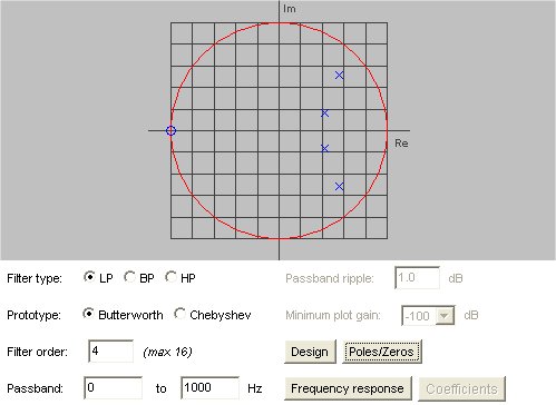 The frequency response is for the range 0 to 4000 Hz based on
the 8000 Hz sampling. 0 db is at the top, the bottom is the
user selected range, -100 db is the default.
The frequency response is for the range 0 to 4000 Hz based on
the 8000 Hz sampling. 0 db is at the top, the bottom is the
user selected range, -100 db is the default.
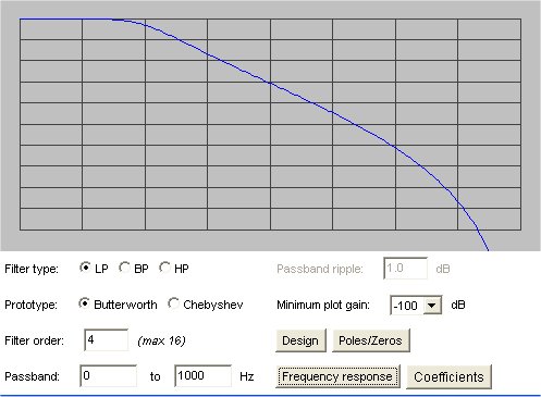 The coefficients are given with zero based subscripts.
(These subscripts may be used directly in C, C++, Java, etc.
add one to the subscript for Fortran, MatLab and diagrams above.)
The coefficients are given with zero based subscripts.
(These subscripts may be used directly in C, C++, Java, etc.
add one to the subscript for Fortran, MatLab and diagrams above.)
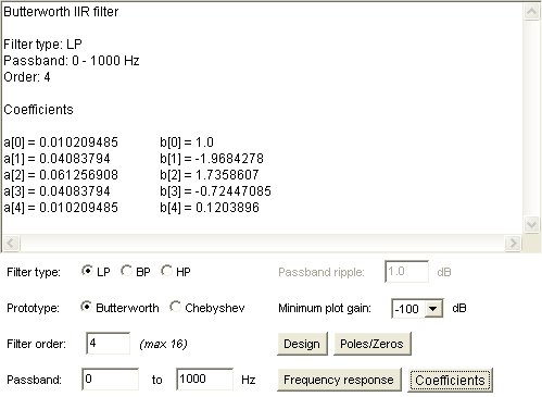 Note that MatLab has 'wavread' and 'wavwrite' functions as well
as a 'sound' function to play .wav files. 'wavwrite' writes
samples at 8000 Hz using the default.
The files to compile and run the Digital Filter coefficients are:
IIRFilterDesign.java
IIRFilter.java
PoleZeroPlot.java
GraphPlot.java
make_filter.bat
Makefile_filter
mydesign.out
This is enough for you to be able to program and use simple
digital filters. This lecture just scratched the surface.
There are many types of digital filters with many variations.
There are complete textbooks on just the subject of digital filters.
The output from the low pass filter shown above "builds up and settles"
quickly:
Note that MatLab has 'wavread' and 'wavwrite' functions as well
as a 'sound' function to play .wav files. 'wavwrite' writes
samples at 8000 Hz using the default.
The files to compile and run the Digital Filter coefficients are:
IIRFilterDesign.java
IIRFilter.java
PoleZeroPlot.java
GraphPlot.java
make_filter.bat
Makefile_filter
mydesign.out
This is enough for you to be able to program and use simple
digital filters. This lecture just scratched the surface.
There are many types of digital filters with many variations.
There are complete textbooks on just the subject of digital filters.
The output from the low pass filter shown above "builds up and settles"
quickly:
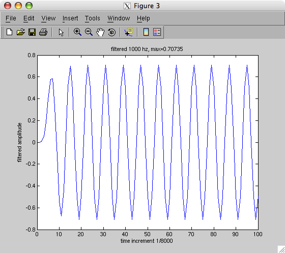 A fourth order band pass filter with band 2000 to 2100 requires
more samples for the center frequency 2050 to build up and settle:
A fourth order band pass filter with band 2000 to 2100 requires
more samples for the center frequency 2050 to build up and settle:
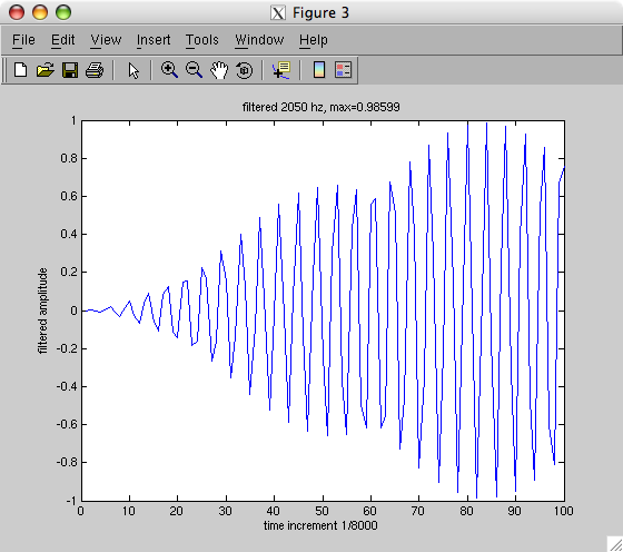 Some notes on db
+3 db is twice the power
-3 db is half the power
+10 db is ten times the power
-10 db is one tenth the power
+30 db is 1000 times the power, 10^3
-30 db is 1/1000 of the power, 10^-3
+60 db is one million times the power, 10^6
-60 db is very small
Sound is measured to average human hearing threshold,
technically 20 micropascals of pressure by definition 0 db.
Some approximate examples for sound from a close source:
0 db threshold of hearing
20 db whisper
60 db normal conversation
80 db vacuum cleaner
90 db lawn mover
110 db front row at rock concert
130 db threshold of pain
140 db military jet takeoff, gun shot, fire cracker
180 db damage to structures
194 db shock waves begin, not normal sound
The sound drops off with distance by the inverse square law.
Each time you move twice as far away from the source,
the sound is 1/4 as strong.
The effective loudness decreases with very short burst of sound.
160 db for 1/100 second is about a loud as 140 db for 1 second.
Sample db vs power code
dbtopower.c source
dbtopower_c.out results
dbtopower.py source
dbtopower_py.out results
Some notes on db
+3 db is twice the power
-3 db is half the power
+10 db is ten times the power
-10 db is one tenth the power
+30 db is 1000 times the power, 10^3
-30 db is 1/1000 of the power, 10^-3
+60 db is one million times the power, 10^6
-60 db is very small
Sound is measured to average human hearing threshold,
technically 20 micropascals of pressure by definition 0 db.
Some approximate examples for sound from a close source:
0 db threshold of hearing
20 db whisper
60 db normal conversation
80 db vacuum cleaner
90 db lawn mover
110 db front row at rock concert
130 db threshold of pain
140 db military jet takeoff, gun shot, fire cracker
180 db damage to structures
194 db shock waves begin, not normal sound
The sound drops off with distance by the inverse square law.
Each time you move twice as far away from the source,
the sound is 1/4 as strong.
The effective loudness decreases with very short burst of sound.
160 db for 1/100 second is about a loud as 140 db for 1 second.
Sample db vs power code
dbtopower.c source
dbtopower_c.out results
dbtopower.py source
dbtopower_py.out results
Many examples of spectra of molecules are presented on the
following pages. The spectra can be used to identify the
presents of specific molecules. Note that the same chemical
designation may result in more than one molecular structure
and the resulting spectra may be different.
Basic physics:
c = velocity of light = about 300,000,000 meters per second
f = frequency in Hz, Kilo KHz = 1000 Hz, Mega Mhz = 106Hz
Giga GHz = 109Hz Tera THz = 1012Hz
λ = wavelength in meters, μ = 10-6 meters = 1000 nano meters
c = λ * f
λ = c / f
f = c / λ
Example: wavelength 1 μ has frequency, f, computed by
f = 300*106 / 10-6 = 300*1012Hz = 300 THz
The "visible" spectrum, that which can be seen by average people,
is roughly given by wavelength in nm = nanometer or 10-9
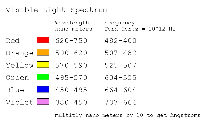 The following pages show the spectrum of many molecules.
The Infrared spectrum has wavelength μ in micrometers, 10-6 meters
The notation Frequency, cm-1 must be multiplied by 30*106
to get Hz.
The Nmr, Nuclear magnetic resonance, data is in Nmr units and Hz.
molecular.pdf Molecular frequency response
The following pages show the spectrum of many molecules.
The Infrared spectrum has wavelength μ in micrometers, 10-6 meters
The notation Frequency, cm-1 must be multiplied by 30*106
to get Hz.
The Nmr, Nuclear magnetic resonance, data is in Nmr units and Hz.
molecular.pdf Molecular frequency response
Go over WEB pages Lecture 11 through 18.
Open book, open notes, no study guide or copy.
Read the instructions.
Follow the instructions, else lose points.
Read the question carefully.
Answer the question that is asked, not the question you want to answer.


Some things you should know:

The roots of a polynomial with real coefficients can be complex.

Some languages have "complex" as a built in type (e.g. Fortran).
Many languages have complex arithmetic available: Ada, Fortran,
MatLab, Mathematica, Python.

Some languages provide standard packages for "complex" (e.g. Ada and C++)

Some languages require you find or make your own "complex" (e.g. C)

All elementary functions are defined and computable for complex arguments.

All complex elementary functions may be computed with only real functions.

Example: sin(z)=sin(re z)*cosh(im z) + i cos(re z)*sinh(im z)

Many languages have either built in or available complex elementary
functions, e.g. Ada, C++, Fortran, Matlab, Mathematica, Java, Python
and some others.

Some complex elementary functions are difficult to compute accurately.

Some elementary functions have a branch cut in the complex plane.

The branch cut is often along the negative real axis.

The derivative is not defined across the branch cut.

Eigenvalues must satisfy several definitions.

There are exactly n eigenvalues for every n by n matrix.

The eigenvalues of a matrix of real elements may be complex.

The determinant of a matrix with a variable subtracted from each
diagonal element yields the characteristic equation of the matrix.
e.g  det|A - eI| = c_n*e^n + ... _ c_1*e + c_0

The roots of the characteristic equation are eigenvalues.

det|A - eI|=0 is one definition of eigenvalues.

Given a polynomial equation, the coefficients of the polynomial may
be placed in a matrix such that the eigenvalues of the matrix are
the roots of the polynomial.

An eigenvector exists for every eigenvalue. Av = ev

It is always possible to find a set of orthogonal eigenvectors
that form the basis of an n dimensional space for an n by n matrix.

Eigenvectors may be complex when the matrix elements and the
eigenvalues are real.

The eigenvectors of a matrix of all ones are usually chosen as the
unit vectors [1 0 ... 0] [0 1 0 ... 0] ... [0 ... 0 1]

The equation  A v = e v must be satisfied for every eigenvalue, e,
and its corresponding eigenvector, v. |v| non zero.

There are many possible test for a program that is supposed to compute
eigenvalues and eigenvectors.

MatLab may not produce unique eigenvectors using [v e]=eig(a)

MatLab may not produce eigenvectors that are mutually orthogonal.

LAPACK is a source of many numerical algorithms implemented in Fortran.

LAPACK code may be converted to any other language.

LAPACK object files may be used with most languages via some interface.

LAPACK source code needs the BLAS, Basic Linear Algebra Subroutines.

The BLAS may be available, optimized, for your computer.

LAPACK is available with files to compile and install on
many computers from  www.netlib.org/lapack

TOMS is numerical source code from the ACM Transactions on Mathematical
software and may be found on www.netlib.org/toms

Some problems require more than double precision floating point.

"gmp" is the gnu multiple precision library of "C" functions.

gmp is available for free download from the Internet.

gmp provides multiple precision integer, rational and floating point.

Any language can implement multi-precision, Java has it available,
other languages use libraries.

52! has too many significant digits to exactly represent in double
precision floating point.

Solving large systems of equation may require multi-precision in order
to get reasonable results.

A simple example of the need for complex roots is x^2+1 = 0
with roots i and -i .

The roots of high order polynomials may be difficult to compute
accurately, e.g. x^16 + 5 = 0 .

There is no algorithm that can guarantee finding all the
roots of every polynomial to a specified accuracy.

Newtons method works most of the time for finding complex roots.
z_next = z - P(z)/P'(z)
(Using a different initial guess usually fixes the problem.)

Optimization is finding the values of independent variables such
that a function is minimized.

Optimizing the absolute value of a function finds the values of
the independent variables that make the function closest to zero.

There is no algorithm that can guarantee finding the optimum
value of every function to a required accuracy.

There are many methods of implementing code to find local minima.
The code varies depending on the assumption of a differentiable
function and on the assumption of no local minima.

The spiral trough is one test case that can be used to test
optimization code.

A Fourier transform of a finite set of data assumes that the
data is repeated infinitely many times before and after the data.

A FFT, Fast Fourier Transform implements a discrete Fourier transform
using order n log n computations for an n point transform. Typically
n must be a power of 2.

The FFT of real data may be complex.

The inverse FFT of the result of and FFT will be reasonably close
to the original data.

The Discrete Fourier transform and FFT of data sampled at time
steps dt will be the frequency spectrum with highest unaliased
frequency 1/(2*dt), the Nyquist frequency.

Digital Filters can be low-pass, high-pass, or band-pass.
A band-pass filter requires two frequencies.
The cutoff frequency is typically 3db down (half power) and
the amplitude decreases faster for higher order filters.

Digital Filters can be described by a set of "a" coefficients
for the numerator and "b" coefficients for the denominator.

Sound power is measured in db, decibel. 0 db for minimum
threshold of hearing. db increases as 10 log10(new_power/old_power)
60 db is 100 times the power of 40 db.

Sound can hurt, 130 db, and greater values may damage buildings.


New applications are happening. Not on the exam,
yet may be of interest:
FFT used on light
Multiple choice and short answer.
No help from other students, that is cheating!

Read quiz carefully. You may think you saw that question
before and know the answer. But, question may have changed.
Dependent and independent are opposite.
"No" or "not" may have been added or deleted.
"some" is different from "all". Numbers can change.

Have all homework 1, 2, 3, 4 finished.
hw4 requires two numbers, both integers, one big 52!

You must download quiz2

last name a-j a, last name k-r b, last name s-z c   ?
cp /afs/umbc.edu/users/s/q/squire/pub/download/q2_455a.doc
cp /afs/umbc.edu/users/s/q/squire/pub/download/q2_455b.doc
cp /afs/umbc.edu/users/s/q/squire/pub/download/q2_455c.doc

Use Microsoft Word  or  libreoffice  to edit.

Then  on linux.gl.umbc.edu
submit cs455 quiz2 q2_455?.doc   or  .docx
A computer benchmark will typically be some code that is executed
and the running time measured.
A few simple rules about benchmarks:
1) Do not believe or trust any person, any company, any data.
2) Expect the same code to give different times on:
different operating systems,
different compilers,
different computers from various manufacturers
(IBM, Sun, Intel, AMD) even at same clock speed,
(IBM Power fastest, AMD next fastest with same memory, cache)
different languages, even for line by line translation.
3) If you want to measure optimization, turn it on,
otherwise prevent all optimization.
(Most compilers provide optimization choices)
(Add code to prevent inlining of functions, force store)
4) You will probably be using your computers clock to measure time.
Test that the clock is giving valid results for the language
you are using. The constant CLOCKS_PER_SEC in the "C" header
file time.h has been found to be wrong.
One manufacturer put a capacitor across the clock circuitry
on a motherboard and all time measurements were half the
correct time. See sample test below.
5) For measuring short times you will need to use the
"double difference method". This method can be used to
measure the time of a single instruction. This method
should be used for any benchmark where one iteration of
the code runs in less than a second. See sample test below.
6) Some methods of measuring time on a computer are only
accurate to one second. Generally run enough iterations of
your code in loops to get a ten second measurement.
Some computers provide a real time clock as accurate as
one microsecond, others one millisecond and some poorer than
a fiftieth of a second.
7) Turn off all networking and stop all software that might run
periodically. If possible, run in single user mode. You want to
measure your code, not a virus checker or operating system.
I once did measurement on a Sun computer running Solaris. It
seemed to slow down periodically. I found that the operating
system periodically checked to see if any disk files needed
to be written.
8) If you are interested in how fast your application might run
on a new computer, find reputable benchmarks that are for
similar applications. I do a lot of numerical computation, thus
all my benchmarks are heavily floating point. You may be
more interested in disk performance or network performance.
9) Do not run all all zero data. Some compilers and very smart and
may precompute your result without running you code.
Be sure to use every result. Compilers do "dead code elimination"
that checks for code where the results are not used and just
does not produce instructions for that "dead code." An "if" test
or printing out the result is typically sufficient. For vectors
and arrays, usually printing out one element is sufficient.
10) It helps to be paranoid. Check that you get the same results
by running n iterations, then 2n iterations. If the time did
not double, you do not have a stable measurement. Run 4n and 8n
and check again. It may not be your benchmark code, it may be
an operating system activity.
11) Do not run a benchmark across midnight. Most computers reset
the seconds to zero at midnight.
12) Keep values of time as a double precision numbers.
13) Given an algorithm where you can predict the time increase
as the size of data increases: e.g. FFT is order n log2 n,
multiplying a matrix by a matrix is order n^3, expect
non uniform results for some values of n.
Consider the case where all your code and all your data fit
in the level one caches. This will be the fastest.
Consider when you data is much larger than the level one cache
yet fits in the level two cache. You are now measuring the
performance of the level two cache.
Consider when your data fits in RAM but is much larger than
your level two (or three) cache. You are now measuring the speed
of your code running in RAM.
Consider when your data is much larger than your RAM, you are
now running in virtual memory from your disk drive. This will
be very slow and you are measuring disk performance.
In order to check the hardware and software time from your computers
clock, run the following two programs. Translate to the language
of your choice. The concept is to have the program display the number
of seconds every 5 seconds for a minute and a half. You check
the display against a watch with a second hand.
The first code uses "clock()" for process time and the second code
uses "time()" for wall clock time.
/* time_cpu.c see if C time.h clock() is OK */
/* in theory, this should be only your processes time */
#include <stdio.h>
#include <time.h>
int main()
{
int i;
double now;
double next;
printf("Should be wall time, 5 second intervals \n");
now = (double)clock()/(double)CLOCKS_PER_SEC;
next = now+5.0;
for(i=0; i<90;)
{
now = (double)clock()/(double)CLOCKS_PER_SEC;
if(now >= next)
{
printf("%d\n",i);
i=i+5;
next=next+5.0;
}
}
return 0;
}
(If time_cpu runs slow, your process is being interrupted.)
time_cpu_c.out
/* time_test.c see if C time.h time(NULL) is OK */
#include <stdio.h>
#include <time.h>
int main()
{
int i;
double now;
double next;
printf("Should be wall time, 5 second intervals \n");
now = (double)time(NULL);
next = now+5.0;
for(i=0; i<90;)
{
now = (double)time(NULL);
if(now >= next)
{
printf("%d\n",i);
i=i+5;
next=next+5.0;
}
}
return 0;
}
time_test_c.out
The "Double Difference Method" tries to get accurate measurement
for very small times. The code to time a single floating point
add instruction is shown below. The principal is:
measure time, t1
run a test harness with loops that has everything except the code
that you want to time. Count the number of executions as a check.
measure time, t2
measure time, t3
run exactly the same code from the test harness with only the
feature you want to measure added. Count number of executions.
measure time, t4
check that the number of executions is the same.
check that t2-t1 was more than 10 seconds
the time for the feature you wanted to measure is
t5 = ((t4 - t3) - (t2 - t1))/ number of executions
basically measured time minus test harness time divided by the
number of executions.
/* time_fadd.c try to measure time of double A = A + B; */
/* roughly time of one floating point add */
/* using double difference and minimum and stability */
#include <time.h>
#include <stdio.h>
#include <math.h>
#define dabs(a) ((a)<0.0?(-(a)):(a))
void do_count(int * count_check, int rep, double * B);
int main(int argc, char * argv[])
{
double t1, t2, t3, t4, tmeas, t_min, t_prev, ts, tavg;
double A, B, Q;
int stable;
int i, j;
int count_check, outer;
int rep, min_rep;
t_min = 10.0; /* 10.0 seconds typical minimum measurement time */
Q = 5.0; /* 5.0 typical approximate percentage stability */
min_rep = 32; /* minimum of 32 typical */
outer = 100000; /* some big number */
printf("time_fadd.c \n");
printf("min time %g seconds, min stability %g percent, outer loop=%d\n",
t_min, Q, outer);
stable = 5; /* max tries */
t_prev = 0.0;
for(rep=min_rep; rep<100000; rep=rep+rep) /* increase until good measure */
{
A = 0.0;
B = 0.1;
t1 = (double)clock()/(double)CLOCKS_PER_SEC;
for(i=0; i<outer; i++) /* outer control loop */
{
count_check = 0;
for(j=0; j<rep; j++) /* inner control loop */
{
do_count(&count_check, rep, &B);
}
}
t2 = (double)clock()/(double)CLOCKS_PER_SEC;
if(count_check != rep) printf("bad count_check_1 %d \n", count_check);
A = 0.0;
t3 = (double)clock()/(double)CLOCKS_PER_SEC;
for(i=0; i<outer; i++) /* outer measurement loop */
{
count_check = 0;
for(j=0; j<rep; j++) /* inner measurement loop */
{
do_count(&count_check, rep, &B);
A = A + B; /* item being measured, approximately FADD time */
}
}
t4 = (double)clock()/(double)CLOCKS_PER_SEC;
if(count_check != rep) printf("bad count_check_2 %d \n", count_check);
tmeas = (t4-t3) - (t2-t1); /* the double difference */
printf("rep=%d, t measured=%g \n", rep, tmeas);
if((t4-t3)<t_min) continue; /* need more rep */
if(t_prev==0.0)
{
printf("tmeas=%g, t_prev=%g, rep=%d \n", tmeas, t_prev, rep);
t_prev = tmeas;
}
else /* compare to previous */
{
printf("tmeas=%g, t_prev=%g, rep=%d \n", tmeas, t_prev, rep);
ts = 2.0*(dabs(tmeas-t_prev)/(tmeas+t_prev));
tavg = 0.5*(tmeas+t_prev);
if(100.0*ts < Q) break; /* above minimum and stable */
t_prev = tmeas;
}
stable--;
if(stable==0) break;
rep = rep/2; /* hold rep constant */
} /* end loop increasing rep */
/* stable? and over minimum */
if(stable==0) printf("rep=%d unstable \n", rep);
if(tmeas<t_min) printf("time measured=%g, under minimum \n", tmeas);
printf("raw time=%g, fadd time=%g, rep=%d, stable=%g\% \n\n", tmeas,
(tavg/(double)outer)/(double)rep, rep, ts);
return 0;
} /* end time_fadd.c */
/* do_count to prevent dead code elimination */
void do_count(int * count_check, int rep, double * B)
{
(*count_check)++;
/* could change B but probably don't have to. */
}
time_fadd_sgi.out
time_fadd_c_sun.out
time_fadd_c_mac.out
You might think that I am obsessed with time. :)
time_cpu.c
time_cpu_c.out
timet_cpu.py3
timet_cpu_py3.out
time_cpu.py3 test
time_test.c
time_test_c.out
time_mp2.c
time_mp2_c.out
time_mp4.c
time_mp4_c.out
time_mp8.c
time_mp8_c.out
time_mp12.c
time_mp12_c.out
time_mp12.c
time_mp12_c.out
time_mp12.c
time_mp12_c.out
time_mp12.c
time_mp12_c.out
time_mp12.c
time_mp12_c.out
fft_time.c
fft_time_a533.out
time_mp2.java
time_mp2_java.out
time_mp4.java
time_mp4_java.out
time_mp8.java
time_mp8_java.out
time_mp12_12.java
time_mp12_12_java.out
time_mp16.java
time_mp16a_java.out
time_mp32.java
time_mp32_java.out
time_mp32a.java
time_mp32a_java.out
time_simeq_thread.java
time_simeq_thread_java.out
time_of_day.java
time_of_day.out
time_cpu.py # python3
time_cpu_py.out
time_test.py
time_test_py.out
time_thread.py
time_thread_py.out
time_cpu.py3
time_cpu_py3.out
time_fadd.py3
time_fadd_py3.out
time_matmul.py3
time_matmul_py3.out
time_matmuln.py3 using numpy
time_matmuln_py3.out
time_test.f90
Many WEB site download/upload speed tests, search or try one:
just click either speed test
64 bit computer architecture
If you have a 64-bit computer and more than 4GB of RAM, here is a
test you may want to run in order to check that your operating
system and compiler are both 64-bit capable:
big_malloc.c
big_malloc.c running, 10 malloc and free 1GB
about to malloc and free 1GB the 1 time
about to malloc and free 1GB the 2 time
about to malloc and free 1GB the 3 time
about to malloc and free 1GB the 4 time
about to malloc and free 1GB the 5 time
about to malloc and free 1GB the 6 time
about to malloc and free 1GB the 7 time
about to malloc and free 1GB the 8 time
about to malloc and free 1GB the 9 time
about to malloc and free 1GB the 10 time
about to malloc and free 2000000000
about to malloc and free 3000000000
about to malloc and free 4000000000
about to malloc and free 5000000000
about to malloc and free 6000000000
about to malloc and free 7000000000
try calloc on 800000000 items of size 8 6.4GB
successful end big_malloc
A 28,000 by 28,000 matrix of double requires about 6.4GB of RAM.
In general, 64-bit is currently supported for the "C" type long
rather than int. Hopefully this will change as most desktop and
laptop computers become 64-bit capable. A small test of various
types and the size in bytes of the types and objects of various
types is:
big.c and its output (older OS)
big.c compiled gcc -m64 -o big big.c (64 bit long)
sizeof(int)=4, sizeof(int1)=4
sizeof(long)=8, sizeof(long1)=8
sizeof(long long)=8, sizeof(llong1)=8
sizeof(float)=4, sizeof(fl1)=4
sizeof(double)=8, sizeof(d1)=8
sizeof(size_t)=8, sizeof(sz1)=8
sizeof(int *)=8, sizeof(p1)=8
n factorial with n of type long
0 ! = 1
1 ! = 1
2 ! = 2
3 ! = 6
4 ! = 24
5 ! = 120
6 ! = 720
7 ! = 5040
8 ! = 40320
9 ! = 362880
10 ! = 3628800
11 ! = 39916800
12 ! = 479001600
13 ! = 6227020800
14 ! = 87178291200
15 ! = 1307674368000
16 ! = 20922789888000
17 ! = 355687428096000
18 ! = 6402373705728000
19 ! = 121645100408832000
20 ! = 2432902008176640000
21 ! = -4249290049419214848 BAD!
22 ! = -1250660718674968576
23 ! = 8128291617894825984
24 ! = -7835185981329244160
big12.c and its output (newer OS)
Note: 'sizeof' change to long, needs %ld rather than %d
big12.c compiled gcc -o big12 big12.c (64 bit long)
-m64 needed on some older OS
sizeof(sizeof(int))=8, sizeof needs pct ld
sizeof(int)=4, sizeof(int1)=4
sizeof(long)=8, sizeof(long1)=8
sizeof(long long)=8, sizeof(llong1)=8
sizeof(float)=4, sizeof(fl1)=4
sizeof(double)=8, sizeof(d1)=8
sizeof(size_t)=8, sizeof(sz1)=8
sizeof(int *)=8, sizeof(p1)=8
n factorial with n of type long (same)
...
trying to malloc 10GB
malloc returned
stored 10GB of 'a'
Some information on the long history of 64-bit computers:
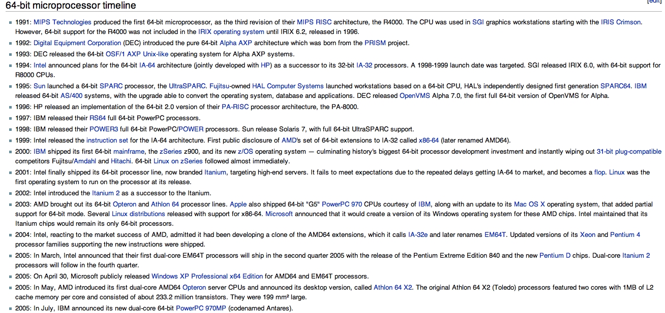 Other code to find out how big an array can be in your
favorite language on your computer:
big_mem.f90 and its output
big_mem.java and its output
big_mem.c and its output
big_mem.adb and its output
Then, more like big_malloc.c, Ada "new"
source code big_new.adb
output from a PC big_new_ada.out
output from a MAC big_new_mac.out
output from a AMD big_new_amd.out
Yes, 50,000 by 50,000 8-byte floating point, not sparse.
20GB of RAM in one matrix.
Now do HW6
Other code to find out how big an array can be in your
favorite language on your computer:
big_mem.f90 and its output
big_mem.java and its output
big_mem.c and its output
big_mem.adb and its output
Then, more like big_malloc.c, Ada "new"
source code big_new.adb
output from a PC big_new_ada.out
output from a MAC big_new_mac.out
output from a AMD big_new_amd.out
Yes, 50,000 by 50,000 8-byte floating point, not sparse.
20GB of RAM in one matrix.
Now do HW6
Project writeup
Use a plotting utility to look at the shape of the function. sample shown
Do a global global search to find candidate staring point, first xbest,ybest.
-1.0 < x < 1.0 -1.0 < y < 1.0 for this project
You need dx, dy of 0.001 to get you into the global minima well.
The global minimum value must be between -3 and -4 by analysis of equation.
You saved best as xbest, ybest, zbest. OK to print.
Top view f(x-dx,y+dy) f(x,y+dy) f(x+dx,y+dy) x is xbest, y is ybest
f(x-dx,y) f(x,y) f(x+dx,y) f(x,y) smallest yet
f(x-dx,y-dy) f(x,y-dy) f(x+dx,y-dy)
Refine from your search result to get a set of eight surrounding
values greater or lower than the zbest value found
refine dx and dy, dx = dx/2, dy=dy/2
example:
*
* |
| | * *
| * | | * |
* | | | | | |
| | | 0 | | | (x+dx,y+dy)
| | | | | | * |
| | | (x,y) | | | (x+dx,y-dy)
| | | | | |
(x-dx,y-dy) | (x,y-dy) (x,y+dy) | (x-dx,y+dy)
| |
(x-dx,y) (x+dx,y)
If none of the 8 z's are smaller, xbest and ybest do not change.
dx = dx/2, dy= dy/2, quit if dx and dy are smaller than desired accuracy.
Use smallest of 8 and adjust xbest,ybest to midpoint between old x,y and
best (x+/-dy, y+/-dy) 8 possible cases.
e.g. (x-dx,y+dy) was smallest:
xbest = xbest-dx
dx = dx/2
ybest = ybest+dy
dy = dy/2
It is OK to print and see progress, typically not at every step.
Or, given a good candidate staring point, use an available minimization
code, typically name "optm" is in file name.
Or, use the previously described expanding and contracting search
that used pseudo derivatives,Lecture 17.
To get high accuracy, 100 digits, requires that the function be
evaluated using multiple precision, covered in an earlier lecture.
Typically, if 100 digit accuracy is desired, then all computation
would be performed at 110 to 200 digit accuracy. This is slow yet
not difficult for sin(x) and exp(x) for small values of x.
exp(x)=1 + x + x^2/2! + x^3/3! + x^4/4! + ...
For |x|<1 you need the nth term where n! > 10^110 or n=75
Or, you can use range reduction and a much shorter series
normalize and use series
e^x = e^j * e^xc integer j, xc = x-j
if xc<1/4 series(xc), if xc<1/2 series(xc/2)^2, else series(xc/4)^4
series 1 + x + x^2/2! + x^3/3! + ... be sure to use multiple precision
Similarly for sin(x) = x - x^3/3! + x^5/5! - x^7/7! + ...
Similarly for cos(x) = 1 - x^2/2! + x^4/4! - x^6/6! + ...
For sqrt(x) make a guess y=1, then iterate y=(y+x/2)/2
until |y-y_previous| < 10^110
Actually, not quite that easy. You must use range reduction
to get |x|<1 and better if |x| < 1/2.
e.g. for sin(x): if abs(x)>2Π then x=x rem 2Π
if x>Π then x=x-2Π
if x<Π then x=x+2Π
if x>Π/2 then x=Π-x
if x<Π/2 then x=Π+x now abs(x)<Π/2 1.57
use sin(x)=2 sin(x/2) cos(x/2) on x/2<Π/4 0.78
Several of the implementations to 200 digits, that I have programmed:
generic_digits_arithmetic.adb
mpf_sin_cos.c
mpf_exp.c
mpf_exp.h
mpf_base.c
mpf_math.h
Big_math.java
test_Big_math.java
Makefile_proj
Obviously, you find a good staring point with global search
using only double precision and
then use a reasonable optimization method to get a good
starting x,y before going to multiple precision computation.
Print, at least the first few, multiple precision values of
x, y, and function and compare to your code that used
double precision floating point. C, Java, Python, Matlab, etc.
Here is why you must do a global search:
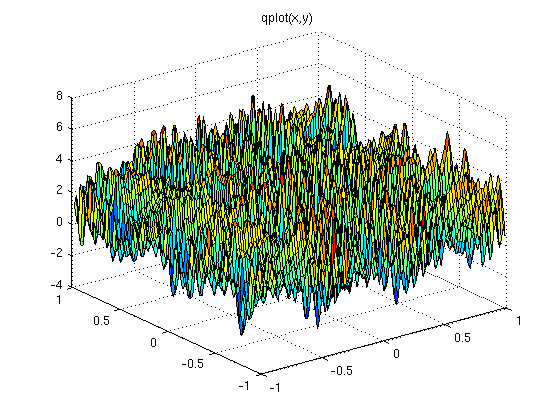 z = exp(sin(50.0*x)) + sin(60.0*exp(y)) +
sin(70.0*sin(x)) + sin(sin(80.0*y)) -
sin(10.0*(x+y)) + (x*x+y*y)/4.0
check you equation when doing project:
for x = -0.0245 y = 0.2105 z should be close to = -3.3067
z = f(x,y) typically set x = xbest, y= ybest, then (x+dx,y) etc.
save z, then zbest = z
When using java, you may need many compilations:
optmn_run.make
Project writeup
Another problem that requires minimation needs physics:
space satellite problem
One possible simple solution:
satellite.java source code
satellite_java.out solution
satellite.py3 source code
satellite_py3.out solution
Could get closer, not needed for launch of satellite.
The function to find the minimum changes every semester.
See project page for this semesters f(x,y)
z = exp(sin(50.0*x)) + sin(60.0*exp(y)) +
sin(70.0*sin(x)) + sin(sin(80.0*y)) -
sin(10.0*(x+y)) + (x*x+y*y)/4.0
check you equation when doing project:
for x = -0.0245 y = 0.2105 z should be close to = -3.3067
z = f(x,y) typically set x = xbest, y= ybest, then (x+dx,y) etc.
save z, then zbest = z
When using java, you may need many compilations:
optmn_run.make
Project writeup
Another problem that requires minimation needs physics:
space satellite problem
One possible simple solution:
satellite.java source code
satellite_java.out solution
satellite.py3 source code
satellite_py3.out solution
Could get closer, not needed for launch of satellite.
The function to find the minimum changes every semester.
See project page for this semesters f(x,y)
Some volumes and areas you should already know:
x1,y1
/\
/ \
x3,y3 /___ \ x2,y2
area of a triangle is 1/2 base times height
| 1 1 1 | | 1 x1 y1 |
area of a triangle is 1/2 det| x1 x2 x3 | = 1/2 det| 1 x2 y2 |
| y1 y2 y3 | | 1 x3 y3 |
area of a triangle is |(V2 - V1) x (V3 - V1)| length of cross product
area of a rectangle is base times height
area of a parallelogram is base times height
area of a circle is Pi r^2
area.txt more area and volume formulas
Some variations that you may need some day:
You may not know the area of a five point star inscribed in
a unit circle or the area of an arbitrary closed polygon.
Easy to calculate, using the Sailors Algorithm:
Given the n points (x,y) of a closed polygon where no edges cross,
compute the sum i=1..n (x_i+1 - x_i) * (y_i+1 + y_i)/2
(The first point is repeated as the n+1 point,
add enough to the y's to make them all positive)
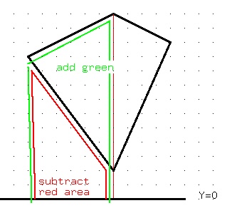 The intuition for the Sailors Algorithm, on a shape with only
vertical and horizontal edges is:
a vertical line adds no area
a horizontal line to the right adds area (length times average height)
a horizontal line to the left subtracts area.
The computed area will be positive if an upper outside edge is
listed in counter clockwise order, else negative, take absolute value.
A sample program is:
area2_dat.py3 source code
star.dat input
area2_dat_py3.out output
poly_area.c
poly_area_maze.out
maze.path
poly_area_star.out
star.path
sailors_area.java
sailors_area_java.out
The maze (8 units wide, 7 units high, area is 35) is:
The intuition for the Sailors Algorithm, on a shape with only
vertical and horizontal edges is:
a vertical line adds no area
a horizontal line to the right adds area (length times average height)
a horizontal line to the left subtracts area.
The computed area will be positive if an upper outside edge is
listed in counter clockwise order, else negative, take absolute value.
A sample program is:
area2_dat.py3 source code
star.dat input
area2_dat_py3.out output
poly_area.c
poly_area_maze.out
maze.path
poly_area_star.out
star.path
sailors_area.java
sailors_area_java.out
The maze (8 units wide, 7 units high, area is 35) is:
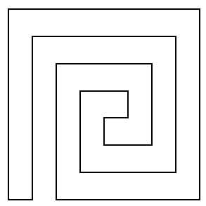 The star (inscribed in a circle with radius 5, area about 28.06) is:
 Volume of a sphere 4/3 Pi r^3
Area of a sphere 4 Pi r^2
Volume of a cone, tetrahedron, any solid with a planar base that goes
to a point 1/3 base area times height
| 1 x1 y1 z1 |
Volume of a tetrahedron 1/6 det | 1 x2 y2 z2 |
| 1 x3 y3 z3 |
| 1 x4 y4 z4 |
using just the x,y,z of the four vertices t1, t2, t3, t4
t4
/\
/ \ missing line from t2 to t4
/ \
/______\
t1\ /t3
\ /
\ /
\/
t2
four surface triangles t1 t2 t3, t1 t2 t4, t1 t3 t4, t2 t3 t4
Volume of a sphere 4/3 Pi r^3
Area of a sphere 4 Pi r^2
Volume of a cone, tetrahedron, any solid with a planar base that goes
to a point 1/3 base area times height
| 1 x1 y1 z1 |
Volume of a tetrahedron 1/6 det | 1 x2 y2 z2 |
| 1 x3 y3 z3 |
| 1 x4 y4 z4 |
using just the x,y,z of the four vertices t1, t2, t3, t4
t4
/\
/ \ missing line from t2 to t4
/ \
/______\
t1\ /t3
\ /
\ /
\/
t2
four surface triangles t1 t2 t3, t1 t2 t4, t1 t3 t4, t2 t3 t4
The general volume computation:
of a closed surface is a little more complicated.
The sailors algorithm is still the basic idea.
Consider a closed surface covered by triangles. Each triangle is
three points and are coded counter clockwise such that the normal
vector to the triangle points out of the volume.
Make all z coordinates positive.
Compute the average z for a triangle, "height".
Compute the area for a triangle, "base".
Compute the z component of the normal vector, znorm.
The volume of this piece of the surface is
height times base times znorm
If znorm is positive, this triangle is on top and contributes
positive volume.
If znorm is negative, this triangle is on the bottom and
contributes negative volume.
The area in the x-y plane is the area of the triangle times znorm.
A vertical triangle has znorm = 0.
A horizontal triangle has znorm = 1 on top and -1 on bottom.
A triangle tipped 45 degrees has a znorm = cos(45 degrees) = 0.7071
znorm is computed using 3 or more points that lie in a plane,
x[0],y[0],z[0] x[1],y[1],z[1] x[2],y[2],z[2] forming
two vectors a and b, then computing the vector cross product:
float znormal(int n, float x[], float y[], float z[], float *area)
{
float ax, ay, az, bx, by, bz, nx, ny, nz, ss;
float cx, cy, cz, sss, sstot, ssstot;
int i;
sstot = 0.0;
ssstot = 0.0;
for(i=2; iNumerical approximation
Using Utah Graphics .dat file for input
volume_dat.py3 source code
volume_dat_py3_cubet.out
volume_dat_py3_tetra.out
tetra.dat input data
cubet.dat input data
A program that uses graphics data files to compute the volume and
area of a closed volume is:
volume_dat2.c
from data:
sphere_div.dat
output for a crude, 32 triangle, sphere is:
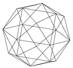 volume_dat2.c reading sphere_div.dat
status=0, zmax=1, points=18, polys=32
xmin=-1.000000, xmax=1.000000, ymin=-1.000000, ymax=1.000000
zmin=-1.000000, zmax=1.000000
enclosing area= 24, enclosing volume= 8
final total area = 10.4178, total volume = 2.94281
should be 12.56 and 4.189
from data:
sphere_div2.dat
output for a better, 128 triangle, sphere is:
volume_dat2.c reading sphere_div2.dat
status=0, zmax=1, points=66, polys=128
xmin=-1.000000, xmax=1.000000, ymin=-1.000000, ymax=1.000000
zmin=-1.000000, zmax=1.000000
enclosing area= 24, enclosing volume= 8
final total area = 11.9549, total volume = 3.81773
should be 12.56 and 4.189
from data:
sphere_div3.dat
output for a better, 512 triangle, sphere is:
volume_dat2.c reading sphere_div3.dat
status=0, zmax=1, points=258, polys=512
xmin=-1.000000, xmax=1.000000, ymin=-1.000000, ymax=1.000000
zmin=-1.000000, zmax=1.000000
enclosing area= 24, enclosing volume= 8
final total area = 12.4082, total volume = 4.0916
should be 12.56 and 4.189
from data:
sphere_div4.dat
output for a good, 2048 triangle, sphere is:
volume_dat2.c reading sphere_div.dat
status=0, zmax=1, points=18, polys=32
xmin=-1.000000, xmax=1.000000, ymin=-1.000000, ymax=1.000000
zmin=-1.000000, zmax=1.000000
enclosing area= 24, enclosing volume= 8
final total area = 10.4178, total volume = 2.94281
should be 12.56 and 4.189
from data:
sphere_div2.dat
output for a better, 128 triangle, sphere is:
volume_dat2.c reading sphere_div2.dat
status=0, zmax=1, points=66, polys=128
xmin=-1.000000, xmax=1.000000, ymin=-1.000000, ymax=1.000000
zmin=-1.000000, zmax=1.000000
enclosing area= 24, enclosing volume= 8
final total area = 11.9549, total volume = 3.81773
should be 12.56 and 4.189
from data:
sphere_div3.dat
output for a better, 512 triangle, sphere is:
volume_dat2.c reading sphere_div3.dat
status=0, zmax=1, points=258, polys=512
xmin=-1.000000, xmax=1.000000, ymin=-1.000000, ymax=1.000000
zmin=-1.000000, zmax=1.000000
enclosing area= 24, enclosing volume= 8
final total area = 12.4082, total volume = 4.0916
should be 12.56 and 4.189
from data:
sphere_div4.dat
output for a good, 2048 triangle, sphere is:
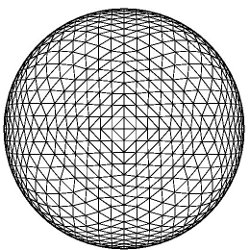 volume_dat2.c reading sphere_div4.dat
status=0, zmax=1, points=1026, polys=2048
xmin=-1.000000, xmax=1.000000, ymin=-1.000000, ymax=1.000000
zmin=-1.000000, zmax=1.000000
enclosing area= 24, enclosing volume= 8
final total area = 12.5264, total volume = 4.16419
should be 12.56 and 4.189
The area of a perfect sphere of radius 1 is about 12.56
The volume of a perfect sphere of radius 1 is about 4.189
from data:
bball.dat Buckminster Fuller Geodesic
output for small, 90 triangle, sphere is:
volume_dat2.c reading sphere_div4.dat
status=0, zmax=1, points=1026, polys=2048
xmin=-1.000000, xmax=1.000000, ymin=-1.000000, ymax=1.000000
zmin=-1.000000, zmax=1.000000
enclosing area= 24, enclosing volume= 8
final total area = 12.5264, total volume = 4.16419
should be 12.56 and 4.189
The area of a perfect sphere of radius 1 is about 12.56
The volume of a perfect sphere of radius 1 is about 4.189
from data:
bball.dat Buckminster Fuller Geodesic
output for small, 90 triangle, sphere is:
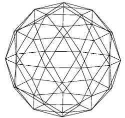 volume_dat2.c reading bball.dat
status=0, zmax=1, points=42, polys=90
xmin=-0.951060, xmax=0.951060, ymin=-1.000000, ymax=1.000000
zmin=-1.000000, zmax=1.000000
enclosing area= 23.217, enclosing volume= 7.60848
final total area = 13.1894, total volume = 3.94159
should be 12.56 and 4.189
No bull? let us compute the volume of this bull
volume_dat2.c reading bball.dat
status=0, zmax=1, points=42, polys=90
xmin=-0.951060, xmax=0.951060, ymin=-1.000000, ymax=1.000000
zmin=-1.000000, zmax=1.000000
enclosing area= 23.217, enclosing volume= 7.60848
final total area = 13.1894, total volume = 3.94159
should be 12.56 and 4.189
No bull? let us compute the volume of this bull
 datread.java needed for volume_dat2
volume_dat2.java program
bull.dat data
volume_dat2.c reading bull.dat
status=0, zmax=3177.82, points=6202, polys=12398
xmin=-2060.574463, xmax=1978.578857, ymin=-1580.072998, ymax=1429.878052
zmin=356.500702, zmax=3177.816406
enclosing area= 6.40908e+07, enclosing volume= 3.43006e+10
final total area = 2.07025e+07, total volume = 3.64616e+09
That's a lot of bull!
Seems scaled up by 500 relative to feet, in all three dimensions.
Thus, about 29.16 cubic feet of bull.
read_stl.java needed for volume_stl
volume_stl.java program
bull.stl data
volume_stl.c reading bull.stl
volume_stl reading file bull.stl
num_tri=12398
xmin=-2060.574463, xmax=1974.23877
ymin=-1580.072998, ymax=1429.878052
zmin=356.500702, zmax=3177.816406
compute volume and area
final total area =2.0702515385253366E7, total volume =3.646510695181979E9
datread.java needed for volume_dat2
volume_dat2.java program
bull.dat data
volume_dat2.c reading bull.dat
status=0, zmax=3177.82, points=6202, polys=12398
xmin=-2060.574463, xmax=1978.578857, ymin=-1580.072998, ymax=1429.878052
zmin=356.500702, zmax=3177.816406
enclosing area= 6.40908e+07, enclosing volume= 3.43006e+10
final total area = 2.07025e+07, total volume = 3.64616e+09
That's a lot of bull!
Seems scaled up by 500 relative to feet, in all three dimensions.
Thus, about 29.16 cubic feet of bull.
read_stl.java needed for volume_stl
volume_stl.java program
bull.stl data
volume_stl.c reading bull.stl
volume_stl reading file bull.stl
num_tri=12398
xmin=-2060.574463, xmax=1974.23877
ymin=-1580.072998, ymax=1429.878052
zmin=356.500702, zmax=3177.816406
compute volume and area
final total area =2.0702515385253366E7, total volume =3.646510695181979E9
Changing volume_dat2.c to volume_ucd.c
Just reading a UCD .inp file, rather than a .dat file.
volume_ucd.c
blivet.inp
volume_ucd_c.out

determining surface normal vectors
The blue dot is on the surface, the red dot is the
direction of the normal.
normal_dat.c
blivet.dat
star3.dat
star3tri.dat
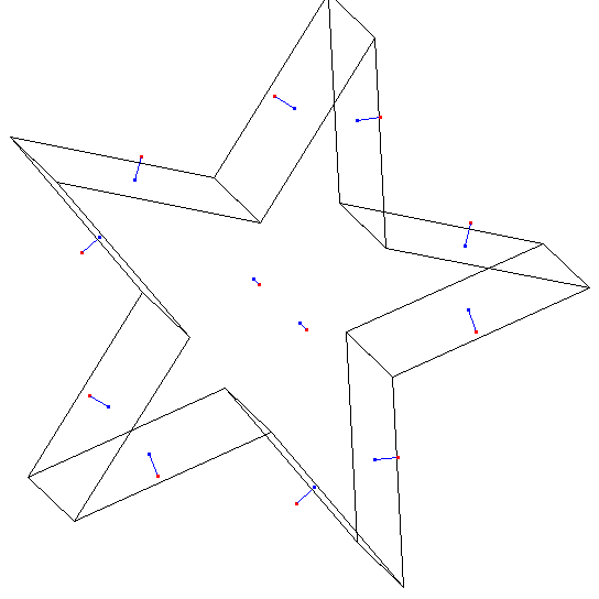
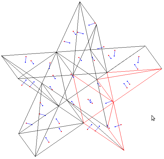 volume_dat2_star3tri.out
More than you every wanted to know about cross product
For 3, 4, 5 etc. dimensions the cross product is a vector in
that dimension that is orthogonal to the given d-1 vectors
in that dimension. The comments, many lines, in the following "C"
program provide definitions, then code provides demonstration.
The checking is that the dot product of two orthogonal vectors
is zero.
cross_general.c comments and source
cross_general_c.out output
cross_general.java comments and source
cross_general_java.out output
simeq_plus.c utility
simeq_plus.h utility
Then, bland 3D versions.
cross_product.c comments and source
cross_product_c.out output
simeq_plus.c utility
simeq_plus.h utility
Then, 6D version, not unique, choice of fill.
cross_product6d.c comments and source
cross_product6d_c.out output
determinant.c utility
determinant.h utility
Then, 6D version, not unique, unit vector fill when less than 5 given.
cross_product6du.c comments and source
cross_product6du_c.out output
determinant.c utility
determinant.h utility
Then there are ellipse, development test to get to ellipse3:
ellipse.java source code
 ellipse.java source code
ellipse.java source code
ellipse_java.out output
ellipse.java source code
ellipse.java source code
ellipse.java source code
ellipse_java.out output
 To determine if a point x,y is inside a closed polygon of lines
test_inside.java source code
test_inside_java.out output
test_meet.java source code
test_meet_java.out output
For sharpening your observation, analyze a few optical illusions:
www.pcmag.com/slideshow/story/325796/14-optical-illusions-that-prove-your-brain-sucks
To determine if a point x,y is inside a closed polygon of lines
test_inside.java source code
test_inside_java.out output
test_meet.java source code
test_meet_java.out output
For sharpening your observation, analyze a few optical illusions:
www.pcmag.com/slideshow/story/325796/14-optical-illusions-that-prove-your-brain-sucks
Numerical differentiation is typically considered poor at best.
In general, high order techniques are needed to get reasonable
values.
Similar to numerical integration, the more values of the function
that are used, then the more accuracy can be expected.
Similar to numerical integration, given a function that can be
fit accurately by an n th order polynomial, an equation for
the derivative exists to give very good accuracy.
Consider a function f(x) that you can compute but do not know
a symbolic representation. To find the derivatives at a few points,
say 4 for example, and computing only 4 evaluations of f(x):
f(x2)
* f(x3)
| *
f(x1) | |
* | |
| | |
f(x0) | | |
* | | |
| | | |
| | | |
x0 x1 x2 x3 h = x3-x2 = x2-x1 = x1-x0
We use f'(x0) to represent the derivative of f(x) at x0.
We looked up the formulas for computing the first derivative
using four equally spaced points, and write the equations:
f'(x0) = 1/6h (-11 f(x0) +18 f(x1) -9 f(x2) 2 f(x3) )
f'(x1) = 1/6h ( -2 f(x0) -3 f(x1) 6 f(x2) -1 f(x3) )
f'(x2) = 1/6h ( 1 f(x0) -6 f(x1) 3 f(x2) 2 f(x3) )
f'(x3) = 1/6h ( -2 f(x0) +9 f(x1) -18 f(x2) 11 f(x3) )
The error estimate is 1/h^4 f''''(z) for worse z in x0..x3
Thus, if the four points are fit by a third degree polynomial,
f''''(z), the fourth derivative is always zero and the numerical
derivatives are exact within roundoff error.
The values will be in an array cx[0]..[3] 1/6h*(-11, 18, -9, 2) .
Then f'(x0) = sum i=0..3 cx[i]*f(x[i])
To check that the coefficients such as -11 18 -9 2 are correct,
we symbolically fit the 4 points with a third order polynomial,
then symbolically take the derivatives. Too much work to do by
hand, thus I used Maple to check and found the coefficients correct.
Using 5 evaluations of f(x) provides the five derivatives:
f'(x0) = 1/12h (-25 f(x0) 48 f(x1) -36 f(x2) 16 f(x3) -3 f(x4) )
f'(x1) = 1/12h ( -3 f(x0) -10 f(x1) 18 f(x2) -6 f(x3) 1 f(x4) )
f'(x2) = 1/12h ( 1 f(x0) -8 f(x1) 0 f(x2) 8 f(x3) -1 f(x4) )
f'(x3) = 1/12h ( -1 f(x0) 6 f(x1) -18 f(x2) 10 f(x3) 3 f(x4) )
f'(x4) = 1/12h ( 3 f(x0) -16 f(x1) 36 f(x2) -48 f(x3) 25 f(x4) )
The above were typed by hand and could have an error.
Some quick checking: If all function evaluations are the same,
then the function is flat and the derivative must be zero at
all points. Thus, the sum of the coefficients must be zero for
every derivative. Note that the first and last coefficients have
the same values, in reverse order with reverse sign.
We will call the "12" in 1/12h the variable b or bb.
We will call the coefficients "-12", "48", "-36" the 'a' array
Always try to cut-and-paste from the computer printout:
Tabulation to compute derivatives at various points
First through sixth order, various number of points
nderiv.out
The above was generated by any of the computer programs listed below:
nderiv.c computes these cases.
nderiv.f90 in Fortran 95
nderiv.adb in Ada 95
nderiv.java in Java
deriv.py in Python 2
rderiv.py in Python 2
nderiv.py in Python 2
deriv.py3 in Python 3
Deriv.scala in Scala
deriv.go in Go language
deriv.jl in Julia
Note that the coefficients can be generated in your program by
copying the function deriv and calling it for a specific
derivative order, number of evaluations and point where derivative
is to be computed. For the second derivative using 4 evaluations
and computing the derivative at point zero,
deriv( 2, 4, 0, a, &bb); returns a={2, -5, 4, -1) and bb=1
thus f''(x0) = 1/bb h^2 ( a[0] f(x0) + a[1] f(x1) + a[2] f(x2) + a[3] f(x3) )
or f''(x0) = 1/h^2 (2 f(x0) -5 f(x0+h) +4 f(x0+2h) -1 f(x0+3h) )
deriv.h header for three versions.
deriv.c computes values.
Note that integers are returned and should be cast to appropriate
floating point type. Various languages require minor changes in the call.
This computation of derivatives will be used extensively in the
lectures that follow on ordinary and partial differential equations.
For non uniformly spaced x values, the program nuderiv.c
demonstrates how to compute the coefficients of f(x0), f(x1), ...
Note that the function nuderiv must be called in the application because
the coefficients depend on the specific problems x values.
The development for non uniformly spaced derivative coefficients is:
given x0, x1, x2, x3 non uniformly spaced
find the coefficients of y0, y1, y2, y3 y0 = f(x0) ...
in order to compute the derivatives:
y'(x0) = c00*y0 + c01*y1 + c02*y2 + c03*y3
y'(x1) = c10*y0 + c11*y1 + c12*y2 + c13*y3
y'(x2) = c20*y0 + c21*y1 + c22*y2 + c23*y3
y'(x3) = c30*y0 + c31*y1 + c32*y2 + c33*y3
Method: fit data to y(x) = a + b*x + c*x^2 + d*x^3
y'(x) = b + 2*c*x + 3*d*x^2
y''(x) = 2*c + 6*d*x
y'''(x) = 6*d
with y0, y1, y2 and y3 variables:
y0 y1 y2 y3
form: | 1 x0 x0^2 x0^3 1 0 0 0 | = a
| 1 x1 x1^2 x1^3 0 1 0 0 | = b
| 1 x2 x2^2 x2^3 0 0 1 0 | = c
| 1 x3 x3^2 x3^3 0 0 0 1 | = d
reduce | 1 0 0 0 a0 a1 a2 a3 | = a
| 0 1 0 0 b0 b1 b2 b3 | = b
| 0 0 1 0 c0 c1 c2 c3 | = c
| 0 0 0 1 d0 d1 d2 d3 | = d
this is just the inverse
y'(x0) = b0*y0 + b1*y1 + b2*y2 + b3*y3 +
2*c0*y0*x0 + 2*c1*y1*x0 + 2*c2*y2*x0 + 2*c3*y3*x0 +
3*d0*y0*x0^2 + 3*d1*y1*x0^2 + 3*d2*y2*x0^2 + 3*d3*y3*x0^2
or c00 = b0 + 2*c0*x0 + 3*d0*x0^2
c01 = b1 + 2*c1*x0 + 3*d1*x0^2
c02 = b2 + 2*c2*x0 + 3*d2*x0^2
c03 = b3 + 2*c3*x0 + 3*d3*x0^2
y'(x0) = c00*y0 + c01*y1 + c02*y2 +c03*y3 where y0 is f(x0) etc.
y'(x1) = b0*y0 + b1*y1 + b2*y2 + b3*y3 +
2*c0*y0*x1 + 2*c1*y1*x1 + 2*c2*y2*x1 + 2*c3*y3*x1 +
3*d0*y0*x1^2 + 3*d1*y1*x1^2 + 3*d2*y2*x1^2 + 3*d3*y3*x1^2
or c10 = b0 + 2*c0*x1 + 3*d0*x1^2
c11 = b1 + 2*c1*x1 + 3*d1*x1^2
c12 = b2 + 2*c2*x1 + 3*d2*x1^2
c13 = b3 + 2*c3*x1 + 3*d3*x1^2
cij = bj + 2*cj*xi + 3*dj*xi^2
y'(x1) = c10*y0 + c11*y1 + c12*y2 +c13*y3
y''(x0) = 2*c0*y0 + 2*c1*y1 + 2*c2*y2 + 2*c3*y3 +
6*d0*y0*x0 + 6*d1*y1*x0 + 6*d2*y2*x0 + 6*d3*y3*x0
or c00 = 2*c0 + 6*d0*x0
c01 = 2*c1 + 6*d1*x0
c02 = 2*c2 + 6*d2*x0
c03 = 2*c3 + 6*d3*x0
y'''(x0) = 6*d0*y0 + 6*d1*y1 + 6*d2*y2 + 6*d3*y3
or c00 = 6*d0 independent of x
c01 = 6*d1
c02 = 6*d2
c03 = 6*d3
The function prototype is
nuderiv.h
void nuderiv(int order, int npoint, int point, double x[], double c[])
where order is the order of the desired derivative
where npoint is the desired number of points (length of x[] and c[] arrays)
where point is desired x index for the derivative
where x[] is input x0, x1, ...
where c[] is output c_point_0, c_point_1, ...
For reasonably smooth functions, using larger numbers of points
allows greater spacing between points and thus fewer equations in
the system of equations to be solved.
Intermediate points may then be found by multidimensional interpolation.
See Lecture 4 for method.
nuderiv.c
nuderiv.h
nuderiv_test.c
nuderiv_test.out
nuderiv.adb
nuderiv_test.adb
nuderiv_test_ada.out
inverse.adb
nuderiv_test_exp.adb
nuderiv_test_exp_ada.out
nuderiv.f90
nuderiv_test.f90
nuderiv_test_f90.out
inverse.f90
nuderiv.java
nuderiv_test.java
nuderiv_test_java.out
test_nuderiv.java
test_nuderiv_java.out
nuderiv.py
nuderiv_test.py
nuderiv_test_py.out
Deriv.scala
TestDeriv.scala
TestDeriv_scala.out
some definitions and explanation of formulas
A test application of nuderiv.c on a 2D PDE that should be exact is
pdenu22_eq.c
pdenu22_eq.out
A test application of nuderiv.adb on a 2D PDE that should be exact is
pdenu22_eq.adb
pdenu22_eq_ada.out
A test application of nuderiv.java on a 2D PDE that should be exact is
pdenu22_eq.java
pdenu22_eq_java.out
A test application of nuderiv.f90 on a 2D PDE that should be exact is
pdenu22_eq.f90
pdenu22_eq_f90.out
A non perfect application to a smooth function exp(x*y)*sin(x+y)
pdenu_eq.c
pdenu_eq.out
pdenu_eq.adb
pdenu_eq_ada.out
pdenu_eq.java
pdenu_eq_java.out
pdenu_eq.f90
pdenu_eq_f90.out
A test application of nuderiv.c on a 3D PDE that should be close is
Note how each term of the differential equation is processed.
This case used 1.0, 2.0, ... for coefficients yet any expression
in x,y,z could be used. A term such as u(x,y,z) * du(x,y,z)/dx
would create a non linear system of equations that would be very
difficult to solve.
pdenu23_eq.c
pdenu23_eq.out
A test application of nuderiv.adb on a 3D PDE that should be close is
pdenu23_eq.adb
pdenu23_eq_ada.out
A test application of nuderiv.f90 on a 3D PDE that should be close is
pdenu23_eq.f90
pdenu23_eq_f90.out
The test code was generated with Maple:
Start by choosing a solution, u(x,y,z) any function of x,y,z.
Symbolically compute the derivatives.
c(x,y,z) is computed as the RHS (right hand side) of the
chosen differential equation, dx(x,y,z) = du(x,y,z)/dx etc.
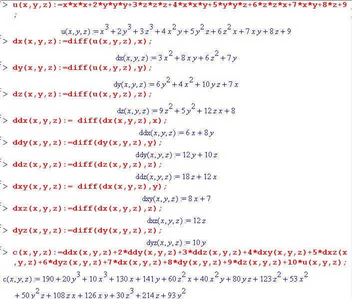 For analytic derivatives see:
derivative.shtml
For analytic derivatives see:
derivative.shtml
Extending derivative computation to partial derivatives uses
the previous work on computing derivatives. Here we consider
the Cartesian coordinate system in 2, 3, and 4 dimensions,
computing second, third and fourth partial derivatives
The algorithms and some code shown below will be used when the
function is unknown, when we are solving partial differential
equations.
Consider a function f(x,y) that you can compute but do not know
a symbolic representation. To find the derivatives at a point
(x,y) we will use our previously discussed "nuderiv" nonuniform
derivative function.
To compute the numerical derivatives of f(x,y) at a set of points
we choose the number of points in the x and y directions, nx, ny.
Thus we have a grid of cells typically programmed as a
two dimensional array.
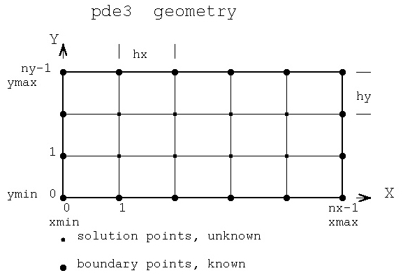 The partial derivative with respect to x at any (x1,y1) point
just uses points (x0,y1) (x1,y1) (x2,y1) ... (xn,y1))
The partial derivative with respect to y at any (x1,y1) point
just uses points (x1,y0) (x1,y1) (x1,y2) ... (x1,yn))
Similarly for second, third, fourth derivatives.
The partial derivative with respect to x and y is more complicated.
We first take the derivative with respect to x, same as calculus.
But, numerically, we need the value for every y.
Then, as in calculus, we take the derivative with respect to y
of the previously computed derivative with respect to x.
(Typically we save the x derivatives as a matrix because we
typically need all the partial derivatives with respect to y.)
A code fragment could look like:
static int nx = 11; /* includes boundary */
static int ny = 10; /* includes boundary */
static double xg[11] = {-1.0, -0.9, -0.8, -0.6, -0.3, 0.0,
0.35, 0.65, 0.85, 1.0, 1.2};
static double yg[10] = {-1.1, -1.0, -0.9, -0.6, -0.2,
0.3, 0.8, 1.0, 1.2, 1.3};
/* nx-2 by ny-2 internal, non boundary cells */
static double cx[11];
static double cy[10];
static double cxy[11][10]; // d^2 u(x,y)/dx dy or Uxy
for(i=1; i<nx-1; i++)
{
for(j=1; j<ny-1; j++) // computing inside boundary
{
/* d^2 u(x,y)/dxdy */
nuderiv(1,nx,i,xg,cx);
nuderiv(1,ny,j,yg,cy);
for(kx=0; k<nx; kx++)
{
for(ky=0; k<ny; ky++)
{
cxy[kx][ky] = cx[kx] * cy[ky]; // numerical derivative at each point
}
}
}
} // have cxy inside the boundary
∂2f(x,y)/∂x ∂y at x=xg[i] y=yg[i] is
computed using coefficients
cxy[kx][ky] = ∂{∂f(x,y)/∂x}/∂y * cx[kx] * cx[ky]
The partial derivative with respect to x at any (x1,y1) point
just uses points (x0,y1) (x1,y1) (x2,y1) ... (xn,y1))
The partial derivative with respect to y at any (x1,y1) point
just uses points (x1,y0) (x1,y1) (x1,y2) ... (x1,yn))
Similarly for second, third, fourth derivatives.
The partial derivative with respect to x and y is more complicated.
We first take the derivative with respect to x, same as calculus.
But, numerically, we need the value for every y.
Then, as in calculus, we take the derivative with respect to y
of the previously computed derivative with respect to x.
(Typically we save the x derivatives as a matrix because we
typically need all the partial derivatives with respect to y.)
A code fragment could look like:
static int nx = 11; /* includes boundary */
static int ny = 10; /* includes boundary */
static double xg[11] = {-1.0, -0.9, -0.8, -0.6, -0.3, 0.0,
0.35, 0.65, 0.85, 1.0, 1.2};
static double yg[10] = {-1.1, -1.0, -0.9, -0.6, -0.2,
0.3, 0.8, 1.0, 1.2, 1.3};
/* nx-2 by ny-2 internal, non boundary cells */
static double cx[11];
static double cy[10];
static double cxy[11][10]; // d^2 u(x,y)/dx dy or Uxy
for(i=1; i<nx-1; i++)
{
for(j=1; j<ny-1; j++) // computing inside boundary
{
/* d^2 u(x,y)/dxdy */
nuderiv(1,nx,i,xg,cx);
nuderiv(1,ny,j,yg,cy);
for(kx=0; k<nx; kx++)
{
for(ky=0; k<ny; ky++)
{
cxy[kx][ky] = cx[kx] * cy[ky]; // numerical derivative at each point
}
}
}
} // have cxy inside the boundary
∂2f(x,y)/∂x ∂y at x=xg[i] y=yg[i] is
computed using coefficients
cxy[kx][ky] = ∂{∂f(x,y)/∂x}/∂y * cx[kx] * cx[ky]
Numerical differentiation can be applied to all coordinate systems.
It gets more complicated, yet a reasonable extension of Cartesian
coordinate systems. These are all partial derivatives.
The algorithms and some code shown below will be used when the
function is unknown, when we are solving partial differential
equations in non Cartesian coordinate systems.
Polar coordinates
Consider a function f(r,theta) that you can compute but do not know
a symbolic representation. To find the derivatives at a point
(r,theta) in a polar coordinate system we will use our previously
discussed "nuderiv" nonuniform Cartesian derivative function.
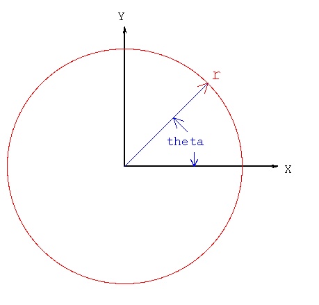 x = r * cos(Θ) r = sqrt(x^2 + y^2) 0 < r
y = r * sin(Θ) Θ = atan2(y,x) 0 ≤ θ < 2Π
^ ^
∇f(r,Θ) = r ∂f/∂r + Θ 1/r ∂f/∂Θ
∇2f(r,Θ) = 1/r ∂/∂r(r*∂f/∂r) + 1/r2 ∂2f/∂Θ2
= 2/r ∂f/∂r + ∂2f/∂r2) + 1/r2 ∂2f/∂Θ2
x = r * cos(Θ) r = sqrt(x^2 + y^2) 0 < r
y = r * sin(Θ) Θ = atan2(y,x) 0 ≤ θ < 2Π
^ ^
∇f(r,Θ) = r ∂f/∂r + Θ 1/r ∂f/∂Θ
∇2f(r,Θ) = 1/r ∂/∂r(r*∂f/∂r) + 1/r2 ∂2f/∂Θ2
= 2/r ∂f/∂r + ∂2f/∂r2) + 1/r2 ∂2f/∂Θ2
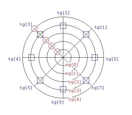 Neither radius grid "rg[]" nor theta grid "tg[]" need to be uniformly
spaced. To compute the derivatives at the green dot, (rg[3],tg[3])
Use the red circle grid points for ∂/∂r and ∂2/∂r2
Use the blue box grid points for ∂/∂Θ and ∂2/∂Θ2
The computation, in "C" language, at rg[3],tg[3] would be:
nuderiv(1, nr, 3, rg, cr); /* nr is 5 in this example */
Ur = 0.0;
for(k=0; k<nr; k++) Ur += cr[k]*f(rg[k],tg[3]); /* ∂/∂r */
nuderiv(1, nt, 3, tg, ct); /* nt is 8 in this sample */
Ut = 0.0;
for(k=0; k<nt; k++) Ut += ct[k]*f(rg[3],tg[k]); /* ∂/∂Θ */
^
nab1r = Ur /* r ∇f(r,Θ) */
^
nab1Θ = (1.0/rg[3])*Ut; /* Θ ∇f(r,Θ) */
nuderiv(2, nr, 3, rg, crr); /* nr is 5 in this example */
Urr = 0.0;
for(k=0; k<nr; k++) Urr += crr[k]*f(rg[k],tg[3]); /* ∂2/∂r2 */
nuderiv(2, nt, 3, tg, ctt); /* nt is 8 in this example */
Utt = 0.0;
for(k=0; k<nt; k++) Utt += ctt[k]*f(rg[3],tg[k]); /* ∂2/∂Θ2 */
nab2 = (2.0/rg[3])*Ur + Urr + (1.0/(rg[3]*rg[3]))*Utt; /* ∇2f(r,Θ) */
The actual code to check these equations at all grid points is:
check_polar_deriv.adb source code
check_polar_deriv_ada.out verification output
Neither radius grid "rg[]" nor theta grid "tg[]" need to be uniformly
spaced. To compute the derivatives at the green dot, (rg[3],tg[3])
Use the red circle grid points for ∂/∂r and ∂2/∂r2
Use the blue box grid points for ∂/∂Θ and ∂2/∂Θ2
The computation, in "C" language, at rg[3],tg[3] would be:
nuderiv(1, nr, 3, rg, cr); /* nr is 5 in this example */
Ur = 0.0;
for(k=0; k<nr; k++) Ur += cr[k]*f(rg[k],tg[3]); /* ∂/∂r */
nuderiv(1, nt, 3, tg, ct); /* nt is 8 in this sample */
Ut = 0.0;
for(k=0; k<nt; k++) Ut += ct[k]*f(rg[3],tg[k]); /* ∂/∂Θ */
^
nab1r = Ur /* r ∇f(r,Θ) */
^
nab1Θ = (1.0/rg[3])*Ut; /* Θ ∇f(r,Θ) */
nuderiv(2, nr, 3, rg, crr); /* nr is 5 in this example */
Urr = 0.0;
for(k=0; k<nr; k++) Urr += crr[k]*f(rg[k],tg[3]); /* ∂2/∂r2 */
nuderiv(2, nt, 3, tg, ctt); /* nt is 8 in this example */
Utt = 0.0;
for(k=0; k<nt; k++) Utt += ctt[k]*f(rg[3],tg[k]); /* ∂2/∂Θ2 */
nab2 = (2.0/rg[3])*Ur + Urr + (1.0/(rg[3]*rg[3]))*Utt; /* ∇2f(r,Θ) */
The actual code to check these equations at all grid points is:
check_polar_deriv.adb source code
check_polar_deriv_ada.out verification output
Cylindrical coordinates
Consider a function f(r,theta,z) that you can compute but do not know
a symbolic representation. To find the derivatives at a point
(r,theta,z) in a cylindrical coordinate system we will use our previously
discussed "nuderiv" nonuniform Cartesian derivative function.
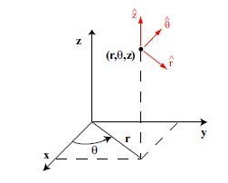 x = r * cos(Θ) r = sqrt(x^2 + y^2 + z^2) 0 < r
y = r * sin(Θ) Θ = atan2(y,x) 0 ≤ θ < 2Π
z = z z = z
^ ^ ^
∇f(r,Θ,z) = r ∂f/∂r + Θ 1/r ∂f/∂Θ + z ∂f/∂z
∇2f(r,Θ,z) = 1/r ∂/∂r(r*∂f/∂r) + 1/r2 ∂2f/∂Θ2 + ∂2f/∂z2
= 2/r ∂f/∂r + ∂2f/∂r2) + 1/r2 ∂2f/∂Θ2 + ∂2f/∂z2
x = r * cos(Θ) r = sqrt(x^2 + y^2 + z^2) 0 < r
y = r * sin(Θ) Θ = atan2(y,x) 0 ≤ θ < 2Π
z = z z = z
^ ^ ^
∇f(r,Θ,z) = r ∂f/∂r + Θ 1/r ∂f/∂Θ + z ∂f/∂z
∇2f(r,Θ,z) = 1/r ∂/∂r(r*∂f/∂r) + 1/r2 ∂2f/∂Θ2 + ∂2f/∂z2
= 2/r ∂f/∂r + ∂2f/∂r2) + 1/r2 ∂2f/∂Θ2 + ∂2f/∂z2
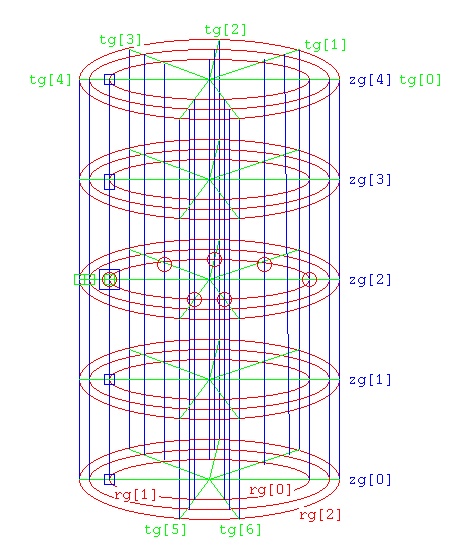 Neither radius grid "rg[]" nor theta grid "tg[]" nor the z grid "zg[]"
need to be uniformly spaced. To compute the derivatives at (rg[0],tg[4],zg[2])
Use the green box grid points for ∂/∂r; and ∂2/∂2r
Use the blue box grid points for ∂2/∂z2
Use the red circle grid points for ∂2/∂Θ2
The computation, in "C" language, would be:
nuderiv(1, nr, 0, rg, cr); /* nr is 3 in this example */
Ur = 0.0;
for(k=0; k<nr; k++) Ur += cr[k]*f(rg[k],tg[4],zg[2]); /* ∂/∂r */
nuderiv(1, nt, 4, tg, ct); /* nt is 7 in this sample */
Ut = 0.0;
for(k=0; k<nt; k++) Ut += ct[k]*f(rg[0],tg[k],zg[2]); /* ∂/∂Θ */
nuderiv(1, nz, 2, zg, cz); /* nz is 5 in this sample */
Uz = 0.0;
for(k=0; k<nz; k++) Uz += cz[k]*f(rg[0],tg[4],zg[k]); /* ∂/∂z */
^
nab1r = Ur /* r ∇f(r,Θ,z) */
^
nab1Θ = (1.0/rg[0])*Ut; /* Θ ∇f(r,&Theta,z) */
^
nab1z = Uz /* z ∇f(r,Θ,z) */
nuderiv(2, nr, 0, rg, crr); /* nr is 3 in this example */
Urr = 0.0;
for(k=0; k<nr; k++) Urr += crr[k]*f(rg[k],tg[4],zg[2]); /* ∂2/∂r2 */
nuderiv(2, nt, 4, tg, ctt); /* nt is 7 in this example */
Utt = 0.0;
for(k=0; k<nt; k++) Utt += ctt[k]*f(rg[0],tg[k],zg[2]); /* ∂2/∂Θ2 */
nuderiv(2, nz, 2, zg, czz); /* nz is 5 in this example */
Uzz = 0.0;
for(k=0; k<nz; k++) Uzz += czz[k]*f(rg[0],tg[4],zg[k]); /* ∂2/∂z2 */
nab2 = (2.0/rg[0])*Ur + Urr + (1.0/(rg[0]*rg[0]))*Utt + Uzz; /* ∇2f(r,Θ,z) */
The actual code to check these equations at all grid points is:
check_cylinder_deriv.adb source code
check_cylinder_deriv_ada.out verification output
Neither radius grid "rg[]" nor theta grid "tg[]" nor the z grid "zg[]"
need to be uniformly spaced. To compute the derivatives at (rg[0],tg[4],zg[2])
Use the green box grid points for ∂/∂r; and ∂2/∂2r
Use the blue box grid points for ∂2/∂z2
Use the red circle grid points for ∂2/∂Θ2
The computation, in "C" language, would be:
nuderiv(1, nr, 0, rg, cr); /* nr is 3 in this example */
Ur = 0.0;
for(k=0; k<nr; k++) Ur += cr[k]*f(rg[k],tg[4],zg[2]); /* ∂/∂r */
nuderiv(1, nt, 4, tg, ct); /* nt is 7 in this sample */
Ut = 0.0;
for(k=0; k<nt; k++) Ut += ct[k]*f(rg[0],tg[k],zg[2]); /* ∂/∂Θ */
nuderiv(1, nz, 2, zg, cz); /* nz is 5 in this sample */
Uz = 0.0;
for(k=0; k<nz; k++) Uz += cz[k]*f(rg[0],tg[4],zg[k]); /* ∂/∂z */
^
nab1r = Ur /* r ∇f(r,Θ,z) */
^
nab1Θ = (1.0/rg[0])*Ut; /* Θ ∇f(r,&Theta,z) */
^
nab1z = Uz /* z ∇f(r,Θ,z) */
nuderiv(2, nr, 0, rg, crr); /* nr is 3 in this example */
Urr = 0.0;
for(k=0; k<nr; k++) Urr += crr[k]*f(rg[k],tg[4],zg[2]); /* ∂2/∂r2 */
nuderiv(2, nt, 4, tg, ctt); /* nt is 7 in this example */
Utt = 0.0;
for(k=0; k<nt; k++) Utt += ctt[k]*f(rg[0],tg[k],zg[2]); /* ∂2/∂Θ2 */
nuderiv(2, nz, 2, zg, czz); /* nz is 5 in this example */
Uzz = 0.0;
for(k=0; k<nz; k++) Uzz += czz[k]*f(rg[0],tg[4],zg[k]); /* ∂2/∂z2 */
nab2 = (2.0/rg[0])*Ur + Urr + (1.0/(rg[0]*rg[0]))*Utt + Uzz; /* ∇2f(r,Θ,z) */
The actual code to check these equations at all grid points is:
check_cylinder_deriv.adb source code
check_cylinder_deriv_ada.out verification output
Spherical coordinates
interchange Φ and Θ on diagram to agree with equations
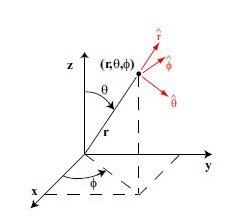 x = r * cos(Θ) * sin(Φ) r = sqrt(x^2 + y^2 + z^2) 0 < r
y = r * sin(Θ) * sin(Φ) Θ = atan2(y,x) 0 ≤ Θ < 2Π
z = r * cos(Φ) Φ = atan2(sqrt(x^2+y^2),z) 0 < Φ < Pi
^ ^ ^
∇f(r,Θ,Φ) = r ∂f/∂r + Θ 1/r sin(Φ) ∂f/∂Θ + Φ 1/r ∂f/∂φ
∇2f(r,Θ,Φ) = 1/r2 ∂/∂r(r2*∂f/∂r) + 1/(r2 sin(Φ)2) ∂2/∂Θ2f + 1/(r2 sin(Φ)) ∂/∂Φ(sin(Φ) ∂/∂f&Phi);
= 2/r ∂f/∂r + ∂2f/∂r2 + 1/(r2 sin(Φ)2) ∂2f/∂Θ2 + cos(Φ)/(r2 sin(Φ)2 ∂f/∂Φ + 1/(r2 ∂2f/∂Φ2
Partial derivatives in R, Theta, Phi follow their color.
All possible are shown.
x = r * cos(Θ) * sin(Φ) r = sqrt(x^2 + y^2 + z^2) 0 < r
y = r * sin(Θ) * sin(Φ) Θ = atan2(y,x) 0 ≤ Θ < 2Π
z = r * cos(Φ) Φ = atan2(sqrt(x^2+y^2),z) 0 < Φ < Pi
^ ^ ^
∇f(r,Θ,Φ) = r ∂f/∂r + Θ 1/r sin(Φ) ∂f/∂Θ + Φ 1/r ∂f/∂φ
∇2f(r,Θ,Φ) = 1/r2 ∂/∂r(r2*∂f/∂r) + 1/(r2 sin(Φ)2) ∂2/∂Θ2f + 1/(r2 sin(Φ)) ∂/∂Φ(sin(Φ) ∂/∂f&Phi);
= 2/r ∂f/∂r + ∂2f/∂r2 + 1/(r2 sin(Φ)2) ∂2f/∂Θ2 + cos(Φ)/(r2 sin(Φ)2 ∂f/∂Φ + 1/(r2 ∂2f/∂Φ2
Partial derivatives in R, Theta, Phi follow their color.
All possible are shown.
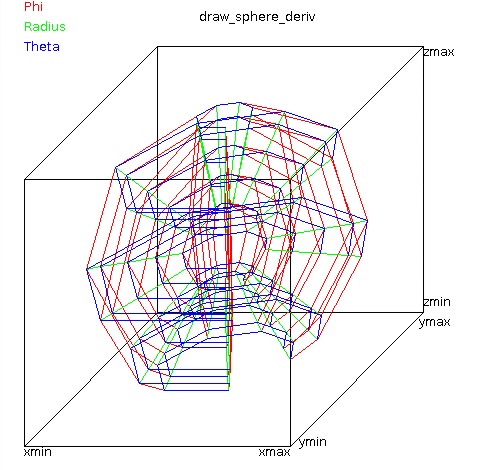 Some "C" code to compute the derivatives at (rg[2],tg[3],zg[4])
nuderiv(2, nr, 2, rg, crr); /* nr is 3 in this example */
Urr = 0.0;
for(k=0; k<nr; k++) Urr += crr[k]*f(rg[k],tg[3],pg[4]); /* ∂2/∂r2 */
nuderiv(2, nt, 3, tg, ctt); /* nt is 7 in this example */
Utt = 0.0;
for(k=0; k<nt; k++) Utt += ctt[k]*f(rg[2],tg[k],pg[4]); /* ∂2/∂Θ2 */
nuderiv(2, np, 4, pg, cpp); /* np is 5 in this example */
Upp = 0.0;
for(k=0; k<np; k++) Upp += cpp[k]*f(rg[2],tg[3],pg[k]); /* ∂2/∂Φ2 */
nab2 = (1.0/rg[0])*Ur + Urr + (1.0/(rg[0]*rg[0]))*Utt + Uzz; /* ∇2f(r,Θ,Φ) */
The actual code to check these equations at all grid points is:
check_sphere_deriv.adb source code
check_sphere_deriv_ada.out verification output
A rather thorough test:
check_spherical_gradient.c source code
check_spherical_gradient_c.out verification output
Other checking of code and one figure came from
draw_sphere_deriv.java
draw_sphere_deriv_java.out
Many functions that do everything with spherical coordinates.
Overboard testing including Laplacian in spherical coordinates.
pde_sphere_mws.out analytic
pde_sphere.c source code
pde_sphere_c.out output
Some "C" code to compute the derivatives at (rg[2],tg[3],zg[4])
nuderiv(2, nr, 2, rg, crr); /* nr is 3 in this example */
Urr = 0.0;
for(k=0; k<nr; k++) Urr += crr[k]*f(rg[k],tg[3],pg[4]); /* ∂2/∂r2 */
nuderiv(2, nt, 3, tg, ctt); /* nt is 7 in this example */
Utt = 0.0;
for(k=0; k<nt; k++) Utt += ctt[k]*f(rg[2],tg[k],pg[4]); /* ∂2/∂Θ2 */
nuderiv(2, np, 4, pg, cpp); /* np is 5 in this example */
Upp = 0.0;
for(k=0; k<np; k++) Upp += cpp[k]*f(rg[2],tg[3],pg[k]); /* ∂2/∂Φ2 */
nab2 = (1.0/rg[0])*Ur + Urr + (1.0/(rg[0]*rg[0]))*Utt + Uzz; /* ∇2f(r,Θ,Φ) */
The actual code to check these equations at all grid points is:
check_sphere_deriv.adb source code
check_sphere_deriv_ada.out verification output
A rather thorough test:
check_spherical_gradient.c source code
check_spherical_gradient_c.out verification output
Other checking of code and one figure came from
draw_sphere_deriv.java
draw_sphere_deriv_java.out
Many functions that do everything with spherical coordinates.
Overboard testing including Laplacian in spherical coordinates.
pde_sphere_mws.out analytic
pde_sphere.c source code
pde_sphere_c.out output
An "ordinary" differential equation has exactly one independent
variable and at least one derivative of that variable.

For notation we use y=f(x) to  say y is a function of x.
For the derivative of y with respect to x, we may write
d f(x)/dx  or we can use  dy/dx  or  y'  when the independent
variable x is understood.

One of the simplest ordinary differential equations is

             y' = y

which has the analytic solution y(x) = exp(x)  the exponential function
also written as e^x .

For a second derivative we use notation d^2 y/dx^2 or y''.

Many ordinary differential equations have analytic solutions. Yet,
many do not. We are interested in ordinary differential equations
that do not have analytic solutions and must be approximated by
numerical solutions. For testing purposes, we will start with an
equation that has an analytic solution so that we can check our
numeric solution method. The test case is the classic beam problem.

given a beam of length L, from 0 < x < L
attached rigidly at both ends
with Young's Modulus of E
with moment of inertia I
with p(x) being the load density  e.g. force per unit length
with both ends fixed, meaning:
      y=0 at x=0, y=0 at x=L, dy/dx=0 at x=0, dy/dx=0 at x=L
then the differential equation that defines the y position of
the beam at every x coordinate is

      d^4 y
   EI ----- = p(x)   with the convention for downward is negative
      dx^4

   for uniformly distributed force (weight) p(x) becomes  - W/L
   This simple case can be integrated and solved analytically:

      d^4 y
   EI ----- = -W/L
      dx^4

     d^3 y
  EI ----- = -W/L x + A   ( A is constant of integration, value found later)
     dx^3

     d^2 y
  EI ----- = -W/L x^2/2 + A x + B
     dx^2

     dy
  EI -- = -W/L x^3/6 + A x^2/2 + B x + C  we see C=0 because dy/dx=0 at x=0
     dx

  EI y = -W/L x^4/24 + A x^3/6 + B x^2/2 + D  we see D=0 because y=0 at x=0

  substituting y=0 at x=L in the equation above gives

     0 = -W/L L^4/24 + A L^3/6 + B L^2/2

  substituting dy/dx=0 at x=L in the equation above the above gives

     0 = -W/L L^3/6 + A L^2/2 + B L

  solving two equations in two unknowns  A = W/2  B = - WL/12
  then substituting for A and B in  EI y = ... and combining terms

         W
  y = --------  x^2 (x-L)^2
      24 L EI

  The known solution for a specific case is valuable to check your
  programming of a numerical solution before computing a more
  general case of p(x) where no closed form solution may exists.

An aside: Much information on physics equations and units and
units conversion may be found in
units.shtml, physics equations near end

In order to find a numerical solution, set up a system of linear
equations such that the solution of the equations are values
of y(x) at some points. The codes below just use seven points, n=7,
yet could use a much larger number. Because we have a fourth order
differential equation, we will use fourth order difference equations.
The solution is fourth order (or less, actually second order) thus
we will get results with no truncation error and only small
roundoff error. The seven points will be equally spaced by h.
h = L/(n+1). The value of y(0)=0 is given and the value y(L)=0
is given. The unknown points are y(h), y(2h), ... , y(7h).

We need the difference equations for fourth order derivatives from
nderiv.out

From nderiv.out the difference equation for d y^4/dx^4
using 5 y values is:

d y^4/dx^4(x) =(1/h^4)( y(x)-4y(x+h)+6y(x+2h)-4y(x+3h)+y(x+4h) )

We will start x at h rather than zero and solve at 7 points.
Since d y^4/dx^4 = -W/L for uniform load, we can get equations
at x=2h ... x=6h. We will need special equations at x=h
and x=7h that take into account the boundary conditions..

  the partial system of equations we want looks like:

  |                             |   | y( h) |   |  0   |
  | -4   6  -4   1   0   0   0  |   | y(2h) |   | -W/L |
  |  1  -4   6  -4   1   0   0  |   | y(3h) |   | -W/L |
  |  0   1  -4   6  -4   1   0  | * | y(4h) | = | -W/L |
  |  0   0   1  -4   6  -4   1  |   | y(5h) |   | -W/L |
  |  0   0   0   1  -4   6  -4  |   | y(6h) |   | -W/L |
  |                             |   | y(7h) |   |  0   |

The boundary conditions dy/dx(0)=0, dy/dx(L)=0
must now be applied. Looking again at nderiv.out for a
first derivative that uses 5 points we find:

dy/dx(x) = 1/12h ( -25y(x) +48y(x+h) -36y(x+2h) +16y(x+3h) -3y(x+4h) )

For x=0, and knowing y(0)=0 we get the first row of the matrix

  | 48 -36  16  -3   0   0   0  |   | y( h) |   |  0   |

At x=L we find

dy/dx(x) = 1/12h ( 3y(x-4h) -16y(x-3h) +36y(x-2h) -48y(x-h) +25y(x) )

For x=L, working backward,  and knowing y(L)=0 we get
the last row of the system of equations.

  | 0   0   0  -3  16 -36  48  |   | y(7h) |   |  0   |

Solve the equations and we have y(h), y(2h), ..., y(7h) as
shown in the output files below in beam2_c.out.

In the code h=1 so that y(h) = y(x=1), y(7h) = y(x=7)
Note that the rather large step size works because we are
using a high enough order method. The analytic solution
is shown with the slopes at each point. The numeric
solution at the end checks very close to the analytic
solution.

beam2.c
beam2_c.out
beam2.f90
beam2_f90.out
beam2.adb
beam2_ada.out
beam2.java
beam2_java.out
beam2.py
beam2_py.out


For more versions of static and dynamic beam equations
Lecture 28d near the end
Quick and dirty numerical solution
Using the notation y for y(x), y' for d y(x)/dx, y'' for d^2 y(x)/dx^2 etc.
To solve a(x) y''' + b(x) y'' + c(x) y' + d(x) y + e(x) = 0
for y at one or more values of x,
with initial condition constants c1, c2, c3 at x0:
y(x0) = c1 y'(x0) = c2 y''(x0) = c3
Create a function that computes y''' =
f(ypp, yp, y, x) = -(b(x)*ypp + c(x)*yp + d(x)*y + e(x))/a(x)
(moving everything except y''' to right-hand-side of equation,
then divide by a(x) )
a(x), b(x), c(x), d(x) and e(x) may be any functions of x and
that includes constants and zero. a(x) must not equal zero in
the range of x0 .. desired largest x.
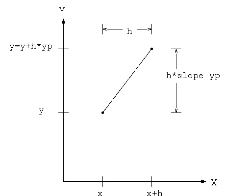 Diagram for y = y + h*yp moving from x to x+h
similarly yp = yp + h*ypp
similarly ypp = ypp + h*yppp
Initialize x = x0
y = c1
yp = c2
ypp = c3
loop: use some method with the function, f, to compute the next ypp
yppp=f(ypp, yp, y, x)
ypp = ypp + h*yppp first order or use some higher order
yp = yp + h*ypp or some higher order method
y = y + h*yp or some higher order method
x = x + h increment x and loop
optional, print y at this x
Quit when you have solved for y at the largest desired x
You may save previous values of x and y, interpolate at desired
value of x to get y.
You may run again with h half as big, keep halving h until you get
approximately the same result.
Quick and dirty finished! This actually works sometimes.
"x" is called the independent variable and
"y" is called the dependent variable.
This is known as an "initial value problem"
The conditions are known at the start and the definition of the
problem is used to numerically compute each successive value of
the solution. This was the method used to compute the flight
of the rocket in homework 1.
Later, we will cover a "boundary value problem" where at least
some information is given at the beginning and end of the
independent variable(s).
Diagram for y = y + h*yp moving from x to x+h
similarly yp = yp + h*ypp
similarly ypp = ypp + h*yppp
Initialize x = x0
y = c1
yp = c2
ypp = c3
loop: use some method with the function, f, to compute the next ypp
yppp=f(ypp, yp, y, x)
ypp = ypp + h*yppp first order or use some higher order
yp = yp + h*ypp or some higher order method
y = y + h*yp or some higher order method
x = x + h increment x and loop
optional, print y at this x
Quit when you have solved for y at the largest desired x
You may save previous values of x and y, interpolate at desired
value of x to get y.
You may run again with h half as big, keep halving h until you get
approximately the same result.
Quick and dirty finished! This actually works sometimes.
"x" is called the independent variable and
"y" is called the dependent variable.
This is known as an "initial value problem"
The conditions are known at the start and the definition of the
problem is used to numerically compute each successive value of
the solution. This was the method used to compute the flight
of the rocket in homework 1.
Later, we will cover a "boundary value problem" where at least
some information is given at the beginning and end of the
independent variable(s).
Better numerical solutions, Runge Kutta
To see some more accurate solutions to very simple ODE's
Solve y' = y y(0)=1 which is just y'(x) = y(x) = exp(x)
Initialize x = 0
y = 1
loop: use yp = y for exp low order method
y = y + h*y yp is just y
x = x + h increment x and loop
print y at this x
Initialize x = 0 Runge Kutta 4th order method
y = 1 this would be exact, within roundoff error,
if solution was 4th order or less polynomial
loop: use yp = y for exp fourth order method for y' = y y=exp(x)
k1 = h*y yp = f(x,y) in general
k2 = h*y+k1/2 f(x+h/2.0,y+k1/2.0)
k3 = h*y+k2/2 f(x+h/2.0,y+k2/2.0)
k4 = h*y+k3 f(x+h,y+k3)
y = y+(k1+2.0*k2+2.0*k3+k4)/6.0
x = x+h print y at this x
rk1_xy_acc.java using RK 4th order
rk1_xy_acc_java.out using RK 4th order
rk1_xy_acc.py3 using RK 4th order
rk1_xy_acc_py3.out using RK 4th order
 ode_exp.c using RK 4th order method
ode_exp_c.out note very small h is worse
To see some more accurate solutions to simple second order ODE's
Solve y'' = -y y(0)=1 y'(0)=0 which is just y(x)= cos(x)
ode_cos.c
ode_cos_c.out many cycles
An example of an unstable ODE is Hopf:
p is a bifurcation parameter, constant for each solution.
Given: dx = gx(x,y,p) = p*x - y - x*(x^2+y^2)
dy = gy(x,y,p) = x + p*y - y*(x^2+y^2)
dr = sqrt(dx^2 + dy^2)
z = f(x,y,p)
Integrate from t=0 to t=tfinal
dz(x,y,p)/dt = dx/dr and
dz(x,y,p)/dt = dy/dr
The plot below uses initial conditions p=-0.1, x=0.4, y=0.4, t=0.0, dt=0.01
and runs to t=10.0
hopf_ode.c
ode_exp.c using RK 4th order method
ode_exp_c.out note very small h is worse
To see some more accurate solutions to simple second order ODE's
Solve y'' = -y y(0)=1 y'(0)=0 which is just y(x)= cos(x)
ode_cos.c
ode_cos_c.out many cycles
An example of an unstable ODE is Hopf:
p is a bifurcation parameter, constant for each solution.
Given: dx = gx(x,y,p) = p*x - y - x*(x^2+y^2)
dy = gy(x,y,p) = x + p*y - y*(x^2+y^2)
dr = sqrt(dx^2 + dy^2)
z = f(x,y,p)
Integrate from t=0 to t=tfinal
dz(x,y,p)/dt = dx/dr and
dz(x,y,p)/dt = dy/dr
The plot below uses initial conditions p=-0.1, x=0.4, y=0.4, t=0.0, dt=0.01
and runs to t=10.0
hopf_ode.c
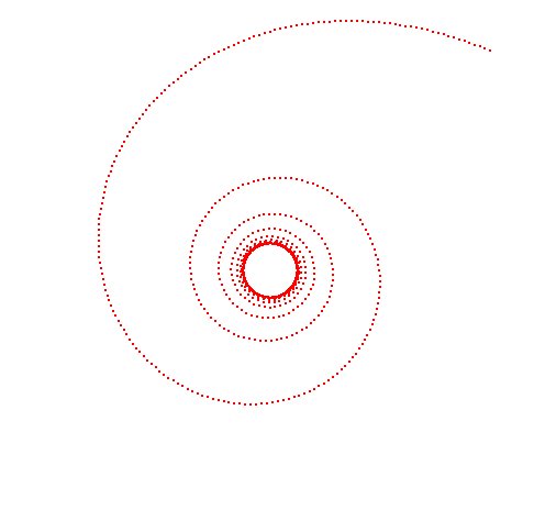 A three body problem, using simple integration, shows the
sling-shot effect of gravity when bodies get close.
Remember force of gravity F = G * mass1 * mass2 / distance^2
This is numerically very unstable.
body3.c needs OpenGL to compile and link.
Hopefully, it can be demonstrated running in class.
body3.java plain Java, different version.
Hopefully, it can be demonstrated running in class.
Center of Mass, Barycenter, general motion
For more typical ordinary differential equations there are some
classic methods. A common higher order method is Runge-Kutta fourth
order.
Given y' = f(x,y) and the initial values of x and y
L: k1 = h * f(x,y)
k2 = h * f(x+h/2.0,y+k1/2.0)
k3 = h * f(x+h/2.0,y+k2/2.0)
k4 = h * f(x+h,y+k3)
y = y + (k1+2.0*k2+2.0*k3+k4)/6.0
x = x + h
quit when x>your_biggest_x
loop to L:
When the solution y(x) is a fourth order polynomial, or lower
order polynomial, the solution will be computed with no truncation
error, yet may have some roundoff error. Very large step sizes, h,
may be used for this very special case.
f(x)=(x-1)*(x-2)*(x-3)*(x-4) 4 roots, and =24 at x=0, x=5
A three body problem, using simple integration, shows the
sling-shot effect of gravity when bodies get close.
Remember force of gravity F = G * mass1 * mass2 / distance^2
This is numerically very unstable.
body3.c needs OpenGL to compile and link.
Hopefully, it can be demonstrated running in class.
body3.java plain Java, different version.
Hopefully, it can be demonstrated running in class.
Center of Mass, Barycenter, general motion
For more typical ordinary differential equations there are some
classic methods. A common higher order method is Runge-Kutta fourth
order.
Given y' = f(x,y) and the initial values of x and y
L: k1 = h * f(x,y)
k2 = h * f(x+h/2.0,y+k1/2.0)
k3 = h * f(x+h/2.0,y+k2/2.0)
k4 = h * f(x+h,y+k3)
y = y + (k1+2.0*k2+2.0*k3+k4)/6.0
x = x + h
quit when x>your_biggest_x
loop to L:
When the solution y(x) is a fourth order polynomial, or lower
order polynomial, the solution will be computed with no truncation
error, yet may have some roundoff error. Very large step sizes, h,
may be used for this very special case.
f(x)=(x-1)*(x-2)*(x-3)*(x-4) 4 roots, and =24 at x=0, x=5
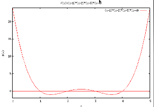 RK4th.java Java example
RK4th_java.out
RK4th.py Python example
RK4th_py.out
RK4th.rb Ruby example
RK4th_ruby.out
RK4th.java Scala example
RK4th_scala.out
In general, the solution will not be accurately approximated by
a low order polynomial. Thus, even the Runge-Kutta method may
require a very small step size in order to compute an accurate
solution. Because very small step sizes result in long computations
and may have large accumulations of roundoff error, variable
step size methods are often used.
Typically a maximum step size and a minimum step size are set.
Starting with some intermediate step size, h, the computation
proceeds as shown below.
Given y' = f(x,y) and the initial values of x and y
L: y1 = y + dy1 using some method with step size h compute dy1
the value of y1 is at x = x + h
y2a = y + dy2a using same method with step size h/2 compute dy2a
the value of y2a is at x = x + h/2
y2 = y2a + dy2 using same method, from y2a at x = x + h/2
with step size h/2 compute dy2
the value of y2 is at x = x + h
abs(y1-y2)>tolerance h = h/2, loop to L:
abs(y1-y2) < tolerance/4 h = 2 * h
y = y2
x = x + h
loop to L: until x > final x
There are many variations on the variable step size method.
The above is one simple version, partially demonstrated by:
FitzHugh-Nagumo equations system of two ODE's
v' = v - v^3/3.0 + r initial v = -1.0
r' = -(v - 0.2 - 0.2*r) initial r = 1.0
initial h = 0.001
t in 0 .. 25
fitz.c just decreasing step size
fitz.out about equally spaced output
fitz.m easier to understand, MatLab
RK4th.java Java example
RK4th_java.out
RK4th.py Python example
RK4th_py.out
RK4th.rb Ruby example
RK4th_ruby.out
RK4th.java Scala example
RK4th_scala.out
In general, the solution will not be accurately approximated by
a low order polynomial. Thus, even the Runge-Kutta method may
require a very small step size in order to compute an accurate
solution. Because very small step sizes result in long computations
and may have large accumulations of roundoff error, variable
step size methods are often used.
Typically a maximum step size and a minimum step size are set.
Starting with some intermediate step size, h, the computation
proceeds as shown below.
Given y' = f(x,y) and the initial values of x and y
L: y1 = y + dy1 using some method with step size h compute dy1
the value of y1 is at x = x + h
y2a = y + dy2a using same method with step size h/2 compute dy2a
the value of y2a is at x = x + h/2
y2 = y2a + dy2 using same method, from y2a at x = x + h/2
with step size h/2 compute dy2
the value of y2 is at x = x + h
abs(y1-y2)>tolerance h = h/2, loop to L:
abs(y1-y2) < tolerance/4 h = 2 * h
y = y2
x = x + h
loop to L: until x > final x
There are many variations on the variable step size method.
The above is one simple version, partially demonstrated by:
FitzHugh-Nagumo equations system of two ODE's
v' = v - v^3/3.0 + r initial v = -1.0
r' = -(v - 0.2 - 0.2*r) initial r = 1.0
initial h = 0.001
t in 0 .. 25
fitz.c just decreasing step size
fitz.out about equally spaced output
fitz.m easier to understand, MatLab
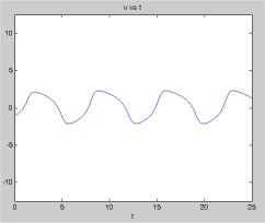
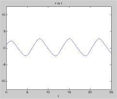 Of course, we can let MatLab solve the same ODE system
fitz2.m using MatLab ode45
The ode45 in MatLab uses a fourth order Runge-Kutta and then
a fifth order Runge-Kutta and compares the result. A neat formulation
is used to minimize the number of required function evaluations.
The fifth order method reuses some of the fourth order evaluations.
Written in "C" from p355 of textbook
fitz2.c similar to fitz.c
fitz2.out close to same results
A second order differential equation use or Runge-Kutta is demonstrated in:
rk4th_second.c
rk4th_second_c.out
A fourth order differential equation use or Runge-Kutta is demonstrated in:
rk4th_fourth.c
rk4th_fourth_c.out
rk4th_fourth.java
rk4th_fourth_java.out
Another coding of fourth order Runge-Kutta known as Gill's method
is the (subroutine, method, function) Runge given in a few languages.
The user provided code comes first, then Runge.
This code solves a system of first order differential equations and
thus can solve higher order differential equations also, as shown above.
Of course, we can let MatLab solve the same ODE system
fitz2.m using MatLab ode45
The ode45 in MatLab uses a fourth order Runge-Kutta and then
a fifth order Runge-Kutta and compares the result. A neat formulation
is used to minimize the number of required function evaluations.
The fifth order method reuses some of the fourth order evaluations.
Written in "C" from p355 of textbook
fitz2.c similar to fitz.c
fitz2.out close to same results
A second order differential equation use or Runge-Kutta is demonstrated in:
rk4th_second.c
rk4th_second_c.out
A fourth order differential equation use or Runge-Kutta is demonstrated in:
rk4th_fourth.c
rk4th_fourth_c.out
rk4th_fourth.java
rk4th_fourth_java.out
Another coding of fourth order Runge-Kutta known as Gill's method
is the (subroutine, method, function) Runge given in a few languages.
The user provided code comes first, then Runge.
This code solves a system of first order differential equations and
thus can solve higher order differential equations also, as shown above.
Systems of ordinary differential equations
The system of differential equations is N equations in N dependent
variables, Y, with one independent variable X.
Y_i = Y'_i(X, Y_1, Y_2, ... , Y_N) for i=1,N
The user provides the code for the functions Y'_i and places
the results in the F array. X goes from initial value, set by user,
to XLIM final value set by user. The user initializes the Y_i.
sim_difeq.f90 Fortran version
sim_difeq_f90.out
sim_difeq.java Java version
sim_difeq_java.out close to same results
sim_difeq.c C version
sim_difeq_c.out close to same results
sim_difeq.m MatLab version (main)
ode_test1.m funct computes derivatives
ode_test4.m funct computes derivatives
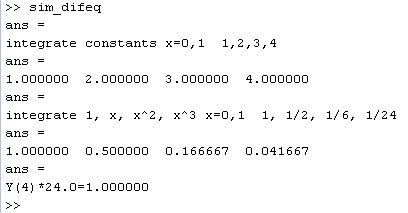
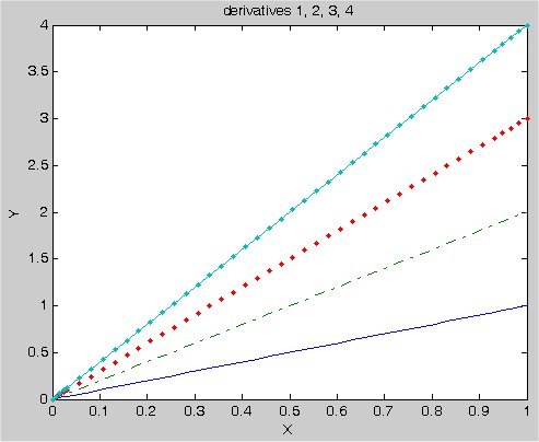
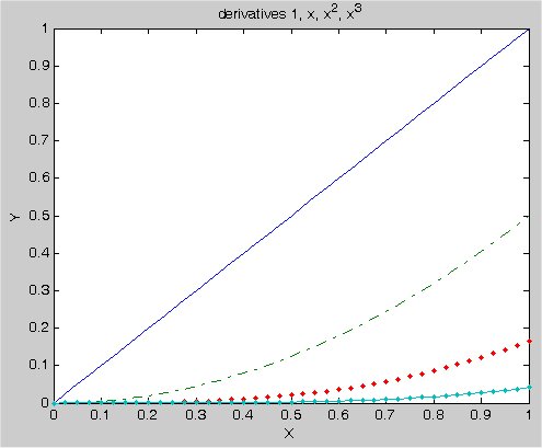
more ordinary differential equations for Matlab solution
ode_1.m sample 1
ode_2.m sample 2
move0.m for sample 2
ode_2a.m sample 2a
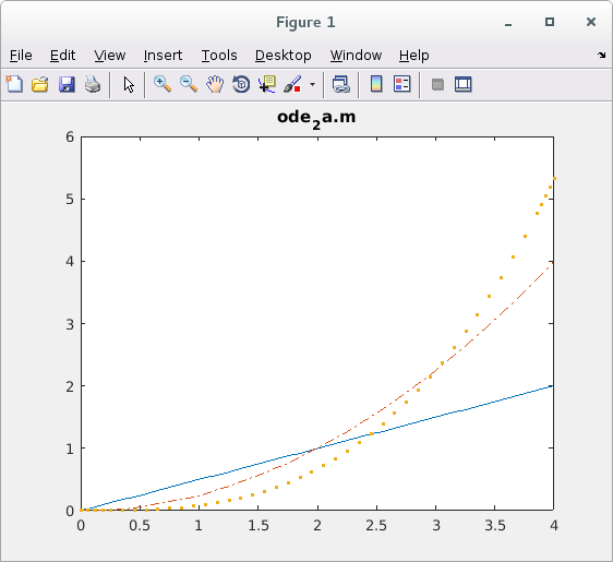 ode_3.m sample 3
ode_4.m sample 4
ode_5.m sample 5
ode_6a.m sample 6
ode_3.m sample 3
ode_4.m sample 4
ode_5.m sample 5
ode_6a.m sample 6
 ode_6a.m sample 6
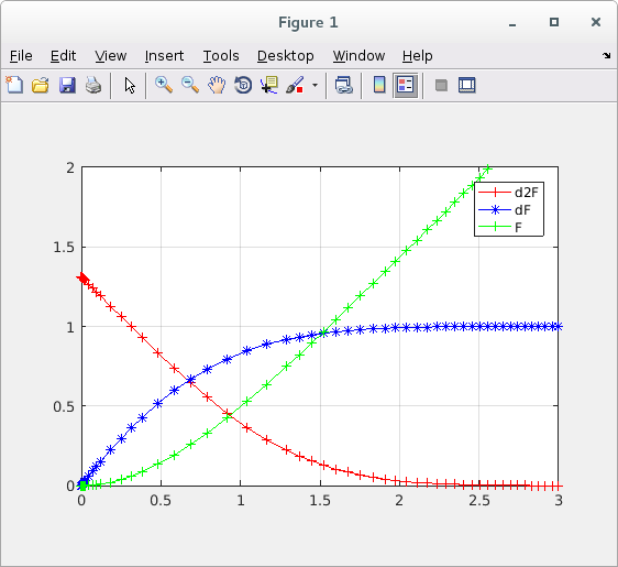 A brief look at definitions (we will cover more later)
See differential equations definitions .
A brief look at definitions (we will cover more later)
See differential equations definitions .
Some partial differential equations are difficult to solve symbolically
and some are difficult to solve numerically.

This lecture covers the numerical solution of simple partial
differential equations where the boundary values are known.

See  simple definitions .

We are told there is an unknown function u(x,y) that satisfies
the partial differential equation:
   (read 'd' as the partial derivative symbol, '^' as exponent)

  d^2u(x,y)/dx^2 + d^2u(x,y)/dy^2 = c(x,y)

and we are given the function c(x,y)
and we are given the values of u(x,y) on the boundary
of the domain of x,y in xmin,ymin to xmax,ymax

To compute the numerical solution of u(x,y) at a set of points
we choose the number of points in the x and y directions, nx, ny.
Thus we have a grid of cells typically programmed as a
two dimensional array.


The number of solution points, unknowns, is typically called
the degrees of freedom, DOF.

From the above we get a step size  hx = (xmax-xmin)/(nx-1) and
hy = (ymax-ymin)/(ny-1). For our first solution we choose
hx = hy = h and just use a step size of h.

If we need u(x,y) at some point not on our solution grid,
we can use two dimensional interpolation to find the desired value.

Now, write the differential equation as a second order
numerical difference equation.
(Numerical derivatives from nderiv.out order 2, points 3, term 1)

d^2u(x,y)/dx^2 + d^2u(x,y)/dy^2 =
 1/h^2(u(x-h,y)-2u(x,y)+u(x+h,y)) +
 1/h^2(u(x,y-h)-2u(x,y)+u(x,y+h)) +O(h^2)

Setting the above equal to c(x,y) and collecting terms

d^2u(x,y)/dx^2 + d^2u(x,y)/dy^2 =  c(x,y) becomes

 1/h^2(u(x-h,y)+u(x+h,y)+u(x,y-h)+u(x,y+h)-4u(x,y))=c(x,y)


now solve for a new u(x,y), based on neighboring grid points
u(x,y)= (u(x-h,y)+u(x+h,0)+u(x,y-h)+u(x,y+h)-c(x,y)*h^2)/4

The formula for u(x,y) is programmed based on indexes i and j
such that x=xmin+i*h, y=ymin+j*h  for i=1,nx-2  j=1,ny-2

Note that the boundary values are set and unchanged for the four
sides  i=0 for j=0,ny-1    i=nx-1 for j=0,ny-1
       j=0 for i=0,nx-1    j=ny-1 for i=0,nx-1
and the interior cells are set to some value, typically zero.

Then iterate, computing new interior cells based on the previous
set of cells including the boundary.

Compute the absolute value of the difference between each new
interior cell and the previous interior cell. A stable problem
will result in this value getting monotonically smaller.

The stopping condition may be based on the above difference
value or on the number of iterations.

To demonstrate the above development, a known u(x,y) is used.
The boundary values are set and the iterations computed.
Since the solution is known, the error can be computed at
each cell and reported for each iteration.

At several iterations, the computed solution and the errors
from the known exact solution are printed.

The same code has been programmed in "C", Java, Fortran 95, Ada 95 and
Matlab as shown below with file types .c, .java, .f90, .adb and .m:


Chose the language you like best and get an understanding of
how the method above was programmed.

"C" source code  pde3.c
output of pde3.c
Fortran 95 source code  pde3.f90
output of pde3.f90
Java source code  pde3.java
output of pde3.java
Ada 95 source code  pde3.adb
output of pde3.adb
Matlab 7 source code  pde3.m
output of pde3.m

You may tailor any of the above code to solve second order
partial differential equations in two independent variables.

1) You need a function  c(x,y)  that is the forcing function, the right
hand side of the differential equation.

2) You need a function  u(x,y)  that provides at least the boundary
conditions. If your  u(x,y)  is not a test solution, remove the "check"
code. And a choice of xmin, xmax, ymin, ymax.

3) If your differential equation is different, then use  nderiv.out
to find the coefficients and create the function  u00(i,j) that
computes the next value of a solution point from the surrounding
previous solution points.

The following examples will be covered for a more general case
in the next lecture. The same problem is solved as given above,
using a method of solving simultaneous linear equations, rather
than an iterative method. The files corresponding to the above
examples are with minimum modifications are:

derivation of  pde3_eq.c
"C" source code  pde3_eq.c
output of pde3_eq.c
Matlab 7 source code  pde3_eq.m
output of pde3_eq.m

Method using solution of simultaneous equations,
rather than an iterative method

Extending to four dimensions in four variables causes the
indexing to get more complex, yet the implementation is
still systematic. An example in C, Java, Ada and Fortran is:
Note that a fourth order method is used when the solution
is at most a fourth order polynomial, thus very small
errors are expected.

"C" source code  pde44_eq.c
output is pde44_eq_c.out
"C" source code  simeq.c
"C" source code  simeq.h
"C" source code  deriv.c
"C" source code  deriv.h

"java" source code  pde44_eq.java
output is pde44_eq_java.out
"java" source code  simeq.java
"java" source code  rderiv.java
"java" source code  test_rderiv.java
output is  test_rderiv_java.out

"Ada" source code  pde44_eq.adb
output is pde44_eq_ada.out
"Ada" source code  pde44h_eq.adb
output is pde44h_eq_ada.out
"Ada" source code  simeq.adb
"Ada" source code  rderiv.adb
"Ada" source code  real_arrays.ads
"Ada" source code  real_arrays.adb

"Fortran" source code  pde44_eq.f90
output is pde44_eq_f90.out
"Fortran" source code  simeq.f90
"Fortran" source code  deriv.f90

"Scala" source code  Pde44_eq.scala
output is Pde44_eq_scala.out
"Scala" source code  Pde44h_eq.scala
output is Pde44h_eq_scala.out
"Scala" source code  Simeq.scala
"Scala" source code  Deriv.scala

Then, the same set using sparse matrix


"C" source code  pde44_sparse.c
output is pde44_sparse_c.out
"C" source code  sparse.c
"C" source code  sparse.h
"C" source code  deriv.c
"C" source code  deriv.h

"java" source code  pde44_sparse.java
output is pde44_sparse_java.out
"java" source code  sparse.java
"java" source code  rderiv.java

"Ada" source code  pde44_sparse.adb
output is pde44_sparse_ada.out
"Ada" source code  sparse1.ads
"Ada" source code  sparse1.adb
"Ada" source code  rderiv.adb
"Ada" source code  real_arrays.ads
"Ada" source code  real_arrays.adb
   (be careful: sparse.ads is zero based subscript,
                sparse1.ads is one based subscript)


The instructor understands that some students have a strong
prejudice in favor of, or against, some programming languages.
After about 50 years of programming in about 17 programming
languages, the instructor finds that the difference between
programming languages is mostly syntactic sugar. Yet, since
students may be able to read some programming languages
easier than others, these examples are presented in "C",
Fortran 90, Java, Ada and Matlab. The intent was to do a quick
translation, keeping most of the source code the same,
for the different languages. Style was not a consideration.
Some rearranging of the order was used when convenient.
In Java and Ada the quick and dirty formatting was used
and thus it is suggested to look at the formatted output of
"C" or Fortran. The numerical results are almost exactly
the same although the presentation differs considerably.
The Matlab code is a combination of "C" and Fortran given
as a single file with internal functions. The subscript base
is shifted from 0 to 1 as in Fortran.

All of this source code compiles and runs on Windows, Linux
and MacOSX. You should not care what operating system your
code will be executed on. Make it operating-system independent.

A very different method, FEM, Finite Element Method
Galerkin FEM overview
Some simplified definitions and terminology related to differential equations:

Given a function  y = f(x)
In plain text, without mathematical symbols, the derivative of
f(x) with respect to x may be written many ways:

  df(x)/dx = df/dx = f'(x) = f'

  or for y=f(x)  dy/dx = y'(x) = y'

  Plain "d" will be used also for the partial derivative symbol.

The fundamental theorem of calculus is:

   Given f(x) is continuous on the interval a <= x <= b and
   F(x) is the indefinite integral of f(x) then
   integral from x=a to x=b of f(x)dx = F(b) - F(a)

Derivative f(x) = dF(x)/dx = F'(x) = F'

   Note that any letters, upper or lower case, may be used for any
   function or variable.

Second Derivative is simply the derivative of the first derivative

   d^2 f(x)/dx^2 = d (df(x)/dx)/dx = f''(x) = f''

Ordinary Differential Equation (ODE)
     A differential equation with only one independent variable.
     Example:  d^2 f(x)/dx^2 = -f(x)  f(0)=0, f'(0)=1 thus  f(x)=sin(x)

Partial Differential Equation (PDE)
     A differential equation with more than one independent variable.
     Example: dU/dx + dU/dy = f(x,y) given f(x,y)=x+y then U(x,y)=xy

Dimension of a differential equation is the number of independent
     variables. Typically the independent variables are:
     x for one dimension
     x,y for two dimensions
     x,y,z for three dimensions
     x,y,z,t for four dimensions, t usually being time.
     x,y,z,u,v,w,t seven independent variables for fluid problems

With many combinations, we use a shorthand, for example for
a function U(x,y,z):
Uxxx is notation for third derivative with respect to x
Uxy  is notation for partial derivative with respect to x and
     with respect to y
Uyzz is notation for partial derivative with respect to y and
     second partial derivative with respect to z


Order of a differential equation is the highest derivative appearing.
     Example: First order:  dF/dx + dF/dy + F(x,y)^3 + x^4 + y^5 = 0
     Example: Second order: d^2 F/dx^2 = F''(x)     Uxx
     Example: Third order:  d^3 F/dx^3 = F'''(x)    Uxxx
     Example: Fourth order: d^4 F/dx^4 = F''''(x)   Uxxxx
     Example: Fourth order: d^4 F/dx^2dydz = F''''(x,y,z) = Uxxyz

Degree of a differential equation is the highest power of any derivatives.
     Example: First degree(linear):  d^2 F/dx^2 + (dF/dx) = 0
     Example: Second degree(quadratic):  (d^3 F/dx^3) + (dF/dx)^2 = 0
     Example: Third degree(cubic):  (d^2 F/dx^2)^3 + (d^4 F/dx^4) = 0
     Example: Third degree: (d^2 F/dxdy)^3 + d^4 F/dxdydzdt = f(x,y,z,t)
     Example: Fourth degree (dF/dx)*(dF/dy)*(dF/dz)*(dF/dt) = 0

     Note: A "linear" differential equation has highest degree one
           for all orders. No U'*U, U^2, U'*U'' etc.
           The solution methods that use solving a linear system of
           equations only work with linear differential equations.
           Higher degree differential equations require solving
           non-linear systems of equations, see Newtons method.

     Note: The Right Hand Side, RHS, is the part to the right of
           the equal sign. This may be zero or a computable function,
           yet must not contain any derivatives or the solution function.
           All derivatives and the solution must be to left of equal sign.
           Example 7*U'(x,y,z)+x*U''(x,y,z)-z*U(x,y,z) = c(x,y,z)^3+x

Initial value differential equation problems have values given at one end
     of the domain.

Boundary value differential equation problems have values given at all ends
     of the domain.
     One dimensional has two values.
     Two dimensional has values on an enclosing path. e.g. square, circle
     Three dimensional has values on an enclosing surface. e.g. cube, sphere
     Four dimensional has values on an enclosing volume. e.g. hyper cube

     Dirichlet boundary values are the values at a point on the boundary.
     Neumann boundary values are the derivative at a point on the boundary,
     typically the first derivative in the direction of the outward normal.

Mixed value partial differential equation problems may have some variables
     initial value and some variables boundary value. Often the time
     variable is given only as an initial value.

Types of second order, first degree, partial differential equations
in two variables, very common, thus named:

  Given  A d^2 U/dx^2 + 2B d^2 U/dxdy + C d^2 U/dy^2 + other terms = f(x,y)

Parabolic  when B^2 = A C   e.g. Diffusion equation
                            one unique real characteristic
                            system has one zero eigenvalue, others
                            all positive or all negative

Elliptic   when B^2 < A C   e.g. Laplace's equation
                            two unique complex characteristics
                            system has eigenvalues all positive or all negative

Hyperbolic when B^2 > A C   e.g. Wave equation
                            two unique real characteristics
                            system has no zero eigenvalues and at least one
                            positive and one negative

    Parabolic Diffusion equation: B=0, C=0
                                  k d^2 V/dx^2 - dV/dt = 0

    Elliptic Laplace's equation:  B=0, A>0, C>0
                                  d^2 V/dx^2 + d^2 V/dy^2 = 0

    Hyperbolic Wave equation:     B=0, A>0, C<0
                                  d^2 V/dx^2 - 1/c^2 d^2 V/dt^2 = 0

The above definitions are motivated by the equation of a cone
cut by a plane at various angles, giving the conic sections:
   parabola,  ellipse  and  hyperbola.

The definitions are extended by some authors to first order
equations such as  dV/dt + a dV/dx = 0 to be called a hyperbolic
one-way wave equation.

The three example equations above are called "homogeneous" because
no term has an independent variable.
More general equations have a forcing function that would replace
the "0" with  f(x,y) or f(x,t) and thus have an inhomogeneous equation.

Using web math symbols:

Laplace Equation is  ΔU = 0  or  ∇2U = 0  or

                     ∂2U/∂x2 + ∂2U/∂y2 + ∂2U/∂z2 = 0

Poisson Equation is  ΔU = f  or  ∇2U = f  or

                     ∂2U/∂x2 + ∂2U/∂y2 + ∂2U/∂z2 = f(x,y,z)


Some terminology is used for various methods of numerical solution
of differential equations.

The Finite Difference Method, FDM, replaces the continuous differential
operators with finite difference approximations. The order of
the approximation may be checked by substitution of the Taylor series.
The FDM is explicit if the solution at the next cell can be expressed
entirely in terms of previously computed cells. Our "nderiv".
The FDM is implicit if the solution at the next group of cells must
be represented as a set of simultaneous equations based on a
previous group of cells.

The Finite Element Method, FEM, develops a system of simultaneous
equations for the solution at every cell.
The FEM is explicit if one solution of the simultaneous equations
yields the solution of the differential equation.
The FEM is iterative if each solution of the simultaneous equations
yields the next approximation to the solution of the differential equation.

more definitions on ODE and PDE
ODE Ordinary Differential Equation - one independent variable
    second order - written many ways:

    a(x)*ΔU  + b(x)*∇U + c(x)*U = f(x)
    a(x)*∇2U + b(x)*∇U + c(x)*U = f(x)
    a(x)*d2U/dx2 + b(x)*dU/dx + c(x)*U = f(x)
    a(x)*U''(x) + b(x)*U'(x) + c(x)*U(x) = f(x)
    a(x)*Uxx(x) + b(x)*Ux(x,y) + c(x)*U(x) = f(x)

    x is independent variable
    the solution is U(x)
    U'(x) is derivative of U(x) with respect to x, written Ux, etc.
    functions a(x), b(x), c(x) and f(x) must be known
    enough initial conditions must be known for a unique solution
    Further definition is needed for choice of coordinate system:
    Cartesian, Cylindrical, Polar, Toroidal, etc.

PDE Partial Differential Equation - more than one independent variable
    a(x,y)*ΔU + b(x,y)*∇U + c(x,y)*ΔU +
    d(x,y)*∇U + e(x,y)*∇U + g(x,y)*U = f(x,y)   ambiguous

    p(x,y)*ΔU + q(x,y)*∇U + r(x,y)*U = f(x,y)   typical

    a(x,y)*∇2U + b(x,y)*∇2U + c(x,y)*∇2U +
    d(x,y)*∇ + e(x,y)*∇U + g(x,y)*U = f(x,y)    ambiguous

    p(x,y)*∇2U + q(x,y)*∇U + r(x,y)*U = f(x,y)    typical

    a(x,y)*∂2U/∂x2 + b(x,y)*∂2U/∂x∂y +
    c(x,y)*∂2U/∂y2 + d(x,y)*∂U/∂x +
    e(x,y)*∂U/∂y + g(x,y)*U = f(x,y)

    a(x,y)*Uxx(x,y) + b(x,y)*Uxy(x,y) + c(x,y)*Uyy(x,y) +
    d(x,y)*Ux(x,y)  + e(x,y)*Uy(x,y)  + g(x,y)*U(x,y) = f(x,y)

    x and y are independent variables
    the solution is U(x,y)
    Ux(x,y) is partial derivative of U(x,y) with respect to x,
    written Ux, Note: U' is ambiguous because it could be Ux or Uy
    Uxy(x,y) is partial derivative of U(x,y) with respect to x and
    partial derivative with respect to y,
    written Uxy,
    functions a(x,y), b(x,y), c(x,y), d(x,y), e(x,y),
    f(x,y) and g(x,y) must be known and computable.
    Enough boundary condition must be known for a unique solution.
    in three dimensions x,y becomes x,y,z
    in four dimensions  x,y becomes x,y,z,t
    in n dimensions the variables are in Rn
    and boundary conditions Ω are given.
    Further definition is needed for choice of coordinate system:
    Cartesian, Cylindrical, Polar, Toroidal, etc.

Methods for computing numerical solutions replace the continuous
variable x with discrete values x1, x2, x3, ... , x_nx
Uniformly spaced values may be used, given xmin, xmax and h,
    xmin, xmin+h, xmin+2h, ... , xmax   nx=1+(xmax-xmin)/h
Discrete values are also used for y, z, and t

The numerical solution is computed at the discrete values of
the independent variables  U(x1), U(x2), U(x3), ... , U(x_nx)
or  U(x1,y1), U(x1,y2), U(x2,y2), ... ,  U(x_nx,y_ny), etc.
The solution is a set of numbers, often written as
U1, U2, ... U_xn  or  U[1,1], U[1,2], U[2,2], ... U[nx,ny]

A numerical solution may use a uniform grid or a
nonuniform grid.

A numerical solution method may be iterative, computing
a closer approximation at each step.

A numerical solution may set up a system of linear equations
to solve for the solution values.

A numerical solution may use a combination of iterative and
linear equations to solve for the solution values.
Not that a non linear differential equation will create a
non linear system of equations to solve. Very difficult!

All of the above statements apply to a set of methods,
generally called discretization.

FEM Finite Element Method is a set of methods for finding the
numerical solution of a differential equation. Within FEM
there are various sub methods including the Galerkin method.

FEM may use equally spaced or variable spaced values for
the independent variables.

FEM may also use triangles, quads, or other polygons for two
independent variables.

FEM may also use tetrahedrons or other solids for three
independent variables. And four dimensional objects for four
independent variables.

see FEM lecture for the rest of the explanation.
cs455_l32.html Finite Element Method
We now extend the analysis and solution to three dimensions and
unequal step sizes.
We are told there is an unknown function u(x,y,z) that satisfies
the partial differential equation:
(read 'd' as the partial derivative symbol, '^' as exponent)
d^2u(x,y,z)/dx^2 + d^2u(x,y,z)/dy^2 + d^2u(x,y,z)/dz^2 = c(x,y,z)
and we are given the function c(x,y,z)
and we are given the values of u(x,y,z) on the boundary
of the domain of x,y,z in xmin,ymin,zmin to xmax,ymax,zmax
To compute the numerical solution of u(x,y,z) at a set of points
we choose the number of points in the x,y and z directions, nx,ny,nz.
The number of non boundary points is called the degrees of freedom, DOF.
Thus we have a grid of cells typically programmed as a
three dimensional array.
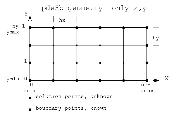 From the above we get a step size hx = (xmax-xmin)/(nx-1) ,
hy = (ymax-ymin)/(ny-1) and hz = (zmax-zmin)/(nz-1).
If we need u(x,y,z) at some point not on our solution grid,
we can use three dimensional interpolation to find the desired value.
Now, write the differential equation as a second order
numerical difference equation. The analytic derivatives are
made discrete by numerical approximation. "Discretization."
(Numerical derivatives from nderiv.out order 2, points 3, term 1)
d^2u(x,y,z)/dx^2 + d^2u(x,y,z)/dy^2 + d^2u(x,y,z)/d^2z =
1/h^2(u(x-h,y,z)-2u(x,y,z)+u(x+h,y,z)) +
1/h^2(u(x,y-h,z)-2u(x,y,z)+u(x,y+h,z)) +
1/h^2(u(x,y,z-h)-2u(x,y,z)+u(x,y,z+h)) + O(h^2)
Setting the above equal to c(x,y,z)
d^2u(x,y,z)/dx^2 + d^2u(x,y,z)/dy^2 + d^2u(x,y,z)/d^2z = c(x,y,z) becomes
1/hx^2(u(x-hx,y,z)+u(x+hx,y,z)-2u(x,y,z)) +
1/hy^2(u(x,y-hy,z)+u(x,y+hy,z)-2u(x,y,z)) +
1/hz^2(u(x,y,z-hz)+u(x,y,z+hz)-2u(x,y,z)) = c(x,y,z)
now solve for new u(x,y,z), based on neighboring grid points
u(x,y,z) = ((u(x-hx,y,z)+u(x+hx,y,z))/hx^2 +
(u(x,y-hy,z)+u(x,y+hy,z))/hy^2 +
(u(x,y,z-hz)+u(x,y,z+hz))/hz^2 - c(x,y,z)) /
(2/hx^2 + 2/hy^2 + 2/hz^2)
The formula for u(x,y,z) is programmed based on indexes i,j,k
such that x=xmin+i*hx, y=ymin+j*hy, z=zmin+k*hz
for i=1,nx-2 j=1,ny-2 k=1,nz-2
Note that the boundary values are set and unchanged for the six
sides i=0 for j=0,ny-1 k=0,nz-1 i=nx-1 for j=0,ny-1 k=0,nz-1
j=0 for i=0,nx-1 k=0,nz-1 j=ny-1 for i=0,nx-1 k=0,nz-1
k=0 for i=0,nx-1 j=0,nx-1 k=nz-1 for i=0,nx-1 j=0,ny-1
and the interior cells are set to some value, typically zero.
Then iterate, computing new interior cells based on the previous
set of cells including the boundary.
Compute the absolute value of the difference between each new
interior cell and the previous interior cell. A stable problem
will result in this value getting monotonically smaller.
The stopping condition may be based on the above difference
value or on the number of iterations.
To demonstrate the above development, a known u(x,y,z) is used.
The boundary values are set and the iterations computed.
Since the solution is known, the error can be computed at
each cell and reported for each iteration.
At several iterations, the computed solution and the errors
from the known exact solution are printed.
The same code has been programmed in "C", Java, Fortran 95 and Ada 95
as shown below with file types .c, .java, .f90 and .adb:
"C" source code pde3b.c
output of pde3b.c
Fortran 95 source code pde3b.f90
output of pde3b.f90
Java source code pde3b.java
output of pde3b.java
Ada 95 source code pde3b.adb
output of pde3b.adb
Matlab 7 source code pde3b.m
output of pde3b.m
It should be noted that a direct solution is possible.
The iterative solution comes from a large set of simultaneous
equations that may be able to be solved accurately. For the
same three dimensional problem above, observe the development
of the set of simultaneous equations:
We are told there is an unknown function u(x,y,z) that satisfies
the partial differential equation:
(read 'd' as the partial derivative symbol, '^' as exponent)
d^2u(x,y,z)/dx^2 + d^2u(x,y,z)/dy^2 + d^2u(x,y,z)/dz^2 = c(x,y,z)
and we are given the function c(x,y,z)
and we are given the values of u(x,y,z) on the boundary ub(x,y,z)
of the domain of x,y,z in xmin,ymin,zmin to xmax,ymax,zmax
To compute the numerical solution of u(x,y,z) at a set of points
we choose the number of points in the x,y and z directions, nx,ny,nz.
Thus we have a grid of cells typically programmed as a
three dimensional array.
From the above we get a step size hx = (xmax-ymin)/(nx-1) ,
hy = (ymax-ymin)/(ny-1) and hz = (xmax-zmin)/(nz-1).
If we need u(x,y,z) at some point not on our solution grid,
we can use three dimensional interpolation to find the desired value.
Now, write the differential equation as a second order
numerical difference equation.
(Numerical derivatives from nderiv.out order 2, points 3, term 1)
d^2u(x,y,z)/dx^2 + d^2u(x,y,z)/dy^2 + d^2u(x,y,z)/d^2z =
1/h^2(u(x-h,y,z)-2u(x,y,z)+u(x+h,y,z)) +
1/h^2(u(x,y-h,z)-2u(x,y,z)+u(x,y+h,z)) +
1/h^2(u(x,y,z-h)-2u(x,y,z)+u(x,y,z+h)) + O(h^2)
Setting the above equal to c(x,y,z)
d^2u(x,y,z)/dx^2 + d^2u(x,y,z)/dy^2 + d^2u(x,y,z)/d^2z = c(x,y,z) becomes
1/hx^2(u(x-hx,y,z)+u(x+hx,y,z)-2u(x,y,z)) +
1/hy^2(u(x,y-hy,z)+u(x,y+hy,z)-2u(x,y,z)) +
1/hz^2(u(x,y,z-hz)+u(x,y,z+hz)-2u(x,y,z)) = c(x,y,z)
Now, rearrange terms to collect the u(x,y,z) coefficients:
u(x-hx,y,z)/hx^2 + u(x+hx,y,z)/hx^2 +
u(x,y-hy,z)/hy^2 + u(x,y+hy,z)/hy^2 +
u(x,y,z-hz)/hz^2 + u(x,y,z+hz)/hz^2 -
u(x,y,z)*(2/hx^2 + 2/hy^2 + 2/hz^2) = c(x,y,z)
We build a linear system of simultaneous equations M U = V
by computing the values of the matrix M and right hand side vector V.
(The system of equations is linear if the differential equation is linear,
otherwise a system of nonlinear equations must be solved.)
The linear subscripts of U corresponding to u(i,j,k) is
m = (i-1)*(ny-2)*(nz-2) + (j-1)*(nz-2) + k
and the rows and columns and V use the same linear subscripts.
Now, using indexes rather than x, x+hx, x-hx,
solve system of linear equations for u(i,j,k).
u(i,j,k)=u(xmin+i*hx, ymin+j*hz, zmin+k*hz)
u(i-1,j,k)/hx^2 + u(i+1,j,k)/hx^2 +
u(i,j-1,k)/hy^2 + u(i,j+1,k)/hy^2 +
u(i,j,k-1)/hz^2 + u(i,j,k+1)/hz^2 -
u(i,j,k)*(2/hx^2 + 2/hy^2 + 2/hz^2) = c(x,y,z)
for i=1,nx-2 j=1,ny-2 k=1,nz-2 while substituting
u(i,j,k) boundary values when i=0 or nx-1, j=0 or ny-1,
k=0 or nz-1 using x=xmin+i*hx, y=ymin+j*hz, z=zmin+k*hz
Remember: hx, hy, hz are known constants, c(x,y,z) is computable.
The matrix has m = (nx-2)*(ny-2)*(nz-2) rows and columns for
solving for m equations in m unknowns. The right hand side vector
is the c(x,y,z) values with possibly boundary terms subtracted.
The unknowns are u(i,j,k) for i=1,nx-2, j=1,ny-2, k=1,nz-2 .
The first row of the matrix is for the unknown u(1,1,1) i=1, j=1, k=1
ub(xmin+0*hx,ymin+1*hy,zmin+1*hz)/hx^2 + u(2,1,1)/hx^2 +
ub(xmin+1*hx,ymin+0*hy,zmin+1*hz)/hy^2 + u(1,2,1)/hy^2 +
ub(xmin+1*hx,ymin+1*hy,zmin+0*hz)/hz^2 + u(1,1,2)/hz^2 +
u(1,1,1)*(2/hx^2 + 2/hy^2 + 2/hz^2) = c(xmin+1*hx,ymin+1*hy,zmin+1*hz)
Matrix cells in first row are zero except for:
M(1,1,1)(1,1,1) = 1/(2/hx^2 + 2/hy^2 + 2/hz^2)
M(1,1,1)(1,1,2) = 1/hz^2
M(1,1,1)(1,2,1) = 1/hy^2
M(1,1,1)(2,1,1) = 1/hx^2
V(1,1,1) = c(xmin+1*hx,ymin+1*hy,zmin+1*hz)
-ub(xmin+0*hx,ymin+1*hy,zmin+1*hz)/hx^2
-ub(xmin+1*hx,ymin+0*hy,zmin+1*hz)/hy^2
-ub(xmin+1*hx,ymin+1*hy,zmin+0*hz)/hz^2
Note that three of the terms are boundary terms and thus have a
computed value that is subtracted from the right hand side vector V.
The row of the matrix for the u(2,2,2) unknown has no boundary terms
u(1,2,2)/hx^2 + u(3,2,2)/hx^2 +
u(2,1,2)/hy^2 + u(2,3,2)/hy^2 +
u(2,2,1)/hz^2 + u(2,2,3)/hz^2 +
u(2,2,2)*(2/hx^2 + 2/hy^2 + 2/hz^2) = c(xmin+2*hx,ymin+2*hy,zmin+2*hz)
Matrix cells in row (2,2,2) are zero except for:
M(2,2,2)(1,2,2) = 1/hx^2
M(2,2,2)(3,2,2) = 1/hx^2
M(2,2,2)(2,1,2) = 1/hy^2
M(2,2,2)(2,3,2) = 1/hy^2
M(2,2,2)(2,2,1) = 1/hz^2
M(2,2,2)(2,2,3) = 1/hz^2
M(2,2,2)(2,2,2) = 1/(2/hx^2 + 2/hy^2 + 2/hz^2)
V(2,2,2) = c(xmin+2*hx,ymin+2*hy,zmin+2*hz)
The number of rows in the matrix is equal to the number of
equations to solve simultaneously and is equal to the
number of unknowns, the degrees of freedom.
The matrix is quite sparse and may be considered "band diagonal".
Typically, special purpose simultaneous equation solvers are
used, often with preconditioners.
A PDE that has all constant coefficients, in this case,
there are only four possible values in the matrix. These are
computed only once at the start of building the matrix.
A PDE with functions of x,y,z as coefficients is covered later.
Solving the system of equations for our test problem gave
the error on the order of 10^-12 compared with
the iterative solution error of 10^-4 after 150 iterations.
The same code has been programmed in "C", Java, Fortran 95, Ada 95 and
Matlab 7 as shown below with file types .c, .java, .f90, .adb and .m:
"C" source code pde3b_eq.c
output of pde3b_eq.c
Fortran 95 source code pde3b_eq.f90
output of pde3b_eq.f90
Java source code pde3b_eq.java
output of pde3b_eq.java
Ada 95 source code pde3b_eq.adb
output of pde3b_eq.adb
Matlab 7 source code pde3b_eq.m
output of pde3b_eq.m
Please note that the solution of partial differential equations
gets significantly more complicated if the solution is not
continuous or is not continuously differentiable.
You can tailor the code presented above for many second order partial
differential equations in three independent variables.
1) You must provide a function u(x,y,z) that computes the solution
on the boundaries. It does not have to be a complete solution and
the "check" code should be removed.
2) You must provide a function c(x,y,z) that computes the
forcing function, the right hand side of the differential equation.
3a) If the differential equation is not d^2/dx^2 + d^2/dy^2 +d^2/dz^2
then use coefficients from nderiv.out to create a new function
u000(i,j,k) that computes a new value of the solution at i,j,k
from the neighboring coordinates for the next iteration.
3b) If the differential equation is not d^2/dx^2 + d^2/dy^2 +d^2/dz^2
then use coefficients from nderiv.out to create a new matrix
initialization function and then solve the simultaneous equations.
3c) There may be constant or function multipliers in the given PDE.
For example exp(x+y/2) * d^2/dx^2 + 7 * d^2/dy^2 etc.
Constant multipliers are just multiplied when creating the
discrete equations. Functions of the independent variables, x,y
must be evaluated at the point where the discrete derivative is
being applied.
For an extended example of discretization of a fourth order PDE
in two dimensions see discrete2d.txt
Source code is available to compute coefficients for derivatives
of many orders. The source code is available in many languages,
deriv.h gives a good overview:
/* deriv.h compute formulas for numerical derivatives */
/* returns npoints values in a or c */
/* 0 <= point < npoints */
void deriv(int order, int npoints, int point, int *a, int *bb);
/* c[point][] = (1.0/((double)bb*h^order))*a[] */
void rderiv(int order, int npoints, int point, double h, double c[]);
/* c includes bb and h^order */
/* derivative of f(x) = c[0]*f(x+(0-point)*h) + */
/* c[1]*f(x+(1-point)*h) + */
/* c[2]*f(x+(2-point)*h) + ... + */
/* c[npoints-1]*f(x+(npoints-1-point)*h */
/* */
/* nuderiv give x values, not uniformly spaced, rather than h */
void nuderiv(int order, int npoints, int point, double x[], double c[]);
deriv.h
deriv.c
deriv.py
deriv.f90
Deriv.scala
deriv.adb
nuderiv.java non uniform, most general
Then the building of the simultaneous equations becomes:
double xg[] = {-1.0, -0.9, -0.8, -0.6, -0.3, 0.0,
0.35, 0.65, 0.85, 1.0, 1.2};
double cxx[] = new double[11]; // nuderiv coefficients
// coefdxx * d^2 u(x,y)/dx^2 for row ii in A matrix
coefdxx = 1.0; // could be a function of xg[i]
new nuderiv(2,nx,i,xg,cxx); // derivative coefficients
for(j=0; j<nx; j++) // cs is index of RHS
{
if(j==0 || j==nx-1)
A[ii][cs] = A[ii][cs] - coefdxx*cxx[j]*ubound(xg[j]);
else A[ii][j] = A[ii][j] + coefdxx*cxx[j];
}
extracted and modified from
pdenu22_eq.java
From the above we get a step size hx = (xmax-xmin)/(nx-1) ,
hy = (ymax-ymin)/(ny-1) and hz = (zmax-zmin)/(nz-1).
If we need u(x,y,z) at some point not on our solution grid,
we can use three dimensional interpolation to find the desired value.
Now, write the differential equation as a second order
numerical difference equation. The analytic derivatives are
made discrete by numerical approximation. "Discretization."
(Numerical derivatives from nderiv.out order 2, points 3, term 1)
d^2u(x,y,z)/dx^2 + d^2u(x,y,z)/dy^2 + d^2u(x,y,z)/d^2z =
1/h^2(u(x-h,y,z)-2u(x,y,z)+u(x+h,y,z)) +
1/h^2(u(x,y-h,z)-2u(x,y,z)+u(x,y+h,z)) +
1/h^2(u(x,y,z-h)-2u(x,y,z)+u(x,y,z+h)) + O(h^2)
Setting the above equal to c(x,y,z)
d^2u(x,y,z)/dx^2 + d^2u(x,y,z)/dy^2 + d^2u(x,y,z)/d^2z = c(x,y,z) becomes
1/hx^2(u(x-hx,y,z)+u(x+hx,y,z)-2u(x,y,z)) +
1/hy^2(u(x,y-hy,z)+u(x,y+hy,z)-2u(x,y,z)) +
1/hz^2(u(x,y,z-hz)+u(x,y,z+hz)-2u(x,y,z)) = c(x,y,z)
now solve for new u(x,y,z), based on neighboring grid points
u(x,y,z) = ((u(x-hx,y,z)+u(x+hx,y,z))/hx^2 +
(u(x,y-hy,z)+u(x,y+hy,z))/hy^2 +
(u(x,y,z-hz)+u(x,y,z+hz))/hz^2 - c(x,y,z)) /
(2/hx^2 + 2/hy^2 + 2/hz^2)
The formula for u(x,y,z) is programmed based on indexes i,j,k
such that x=xmin+i*hx, y=ymin+j*hy, z=zmin+k*hz
for i=1,nx-2 j=1,ny-2 k=1,nz-2
Note that the boundary values are set and unchanged for the six
sides i=0 for j=0,ny-1 k=0,nz-1 i=nx-1 for j=0,ny-1 k=0,nz-1
j=0 for i=0,nx-1 k=0,nz-1 j=ny-1 for i=0,nx-1 k=0,nz-1
k=0 for i=0,nx-1 j=0,nx-1 k=nz-1 for i=0,nx-1 j=0,ny-1
and the interior cells are set to some value, typically zero.
Then iterate, computing new interior cells based on the previous
set of cells including the boundary.
Compute the absolute value of the difference between each new
interior cell and the previous interior cell. A stable problem
will result in this value getting monotonically smaller.
The stopping condition may be based on the above difference
value or on the number of iterations.
To demonstrate the above development, a known u(x,y,z) is used.
The boundary values are set and the iterations computed.
Since the solution is known, the error can be computed at
each cell and reported for each iteration.
At several iterations, the computed solution and the errors
from the known exact solution are printed.
The same code has been programmed in "C", Java, Fortran 95 and Ada 95
as shown below with file types .c, .java, .f90 and .adb:
"C" source code pde3b.c
output of pde3b.c
Fortran 95 source code pde3b.f90
output of pde3b.f90
Java source code pde3b.java
output of pde3b.java
Ada 95 source code pde3b.adb
output of pde3b.adb
Matlab 7 source code pde3b.m
output of pde3b.m
It should be noted that a direct solution is possible.
The iterative solution comes from a large set of simultaneous
equations that may be able to be solved accurately. For the
same three dimensional problem above, observe the development
of the set of simultaneous equations:
We are told there is an unknown function u(x,y,z) that satisfies
the partial differential equation:
(read 'd' as the partial derivative symbol, '^' as exponent)
d^2u(x,y,z)/dx^2 + d^2u(x,y,z)/dy^2 + d^2u(x,y,z)/dz^2 = c(x,y,z)
and we are given the function c(x,y,z)
and we are given the values of u(x,y,z) on the boundary ub(x,y,z)
of the domain of x,y,z in xmin,ymin,zmin to xmax,ymax,zmax
To compute the numerical solution of u(x,y,z) at a set of points
we choose the number of points in the x,y and z directions, nx,ny,nz.
Thus we have a grid of cells typically programmed as a
three dimensional array.
From the above we get a step size hx = (xmax-ymin)/(nx-1) ,
hy = (ymax-ymin)/(ny-1) and hz = (xmax-zmin)/(nz-1).
If we need u(x,y,z) at some point not on our solution grid,
we can use three dimensional interpolation to find the desired value.
Now, write the differential equation as a second order
numerical difference equation.
(Numerical derivatives from nderiv.out order 2, points 3, term 1)
d^2u(x,y,z)/dx^2 + d^2u(x,y,z)/dy^2 + d^2u(x,y,z)/d^2z =
1/h^2(u(x-h,y,z)-2u(x,y,z)+u(x+h,y,z)) +
1/h^2(u(x,y-h,z)-2u(x,y,z)+u(x,y+h,z)) +
1/h^2(u(x,y,z-h)-2u(x,y,z)+u(x,y,z+h)) + O(h^2)
Setting the above equal to c(x,y,z)
d^2u(x,y,z)/dx^2 + d^2u(x,y,z)/dy^2 + d^2u(x,y,z)/d^2z = c(x,y,z) becomes
1/hx^2(u(x-hx,y,z)+u(x+hx,y,z)-2u(x,y,z)) +
1/hy^2(u(x,y-hy,z)+u(x,y+hy,z)-2u(x,y,z)) +
1/hz^2(u(x,y,z-hz)+u(x,y,z+hz)-2u(x,y,z)) = c(x,y,z)
Now, rearrange terms to collect the u(x,y,z) coefficients:
u(x-hx,y,z)/hx^2 + u(x+hx,y,z)/hx^2 +
u(x,y-hy,z)/hy^2 + u(x,y+hy,z)/hy^2 +
u(x,y,z-hz)/hz^2 + u(x,y,z+hz)/hz^2 -
u(x,y,z)*(2/hx^2 + 2/hy^2 + 2/hz^2) = c(x,y,z)
We build a linear system of simultaneous equations M U = V
by computing the values of the matrix M and right hand side vector V.
(The system of equations is linear if the differential equation is linear,
otherwise a system of nonlinear equations must be solved.)
The linear subscripts of U corresponding to u(i,j,k) is
m = (i-1)*(ny-2)*(nz-2) + (j-1)*(nz-2) + k
and the rows and columns and V use the same linear subscripts.
Now, using indexes rather than x, x+hx, x-hx,
solve system of linear equations for u(i,j,k).
u(i,j,k)=u(xmin+i*hx, ymin+j*hz, zmin+k*hz)
u(i-1,j,k)/hx^2 + u(i+1,j,k)/hx^2 +
u(i,j-1,k)/hy^2 + u(i,j+1,k)/hy^2 +
u(i,j,k-1)/hz^2 + u(i,j,k+1)/hz^2 -
u(i,j,k)*(2/hx^2 + 2/hy^2 + 2/hz^2) = c(x,y,z)
for i=1,nx-2 j=1,ny-2 k=1,nz-2 while substituting
u(i,j,k) boundary values when i=0 or nx-1, j=0 or ny-1,
k=0 or nz-1 using x=xmin+i*hx, y=ymin+j*hz, z=zmin+k*hz
Remember: hx, hy, hz are known constants, c(x,y,z) is computable.
The matrix has m = (nx-2)*(ny-2)*(nz-2) rows and columns for
solving for m equations in m unknowns. The right hand side vector
is the c(x,y,z) values with possibly boundary terms subtracted.
The unknowns are u(i,j,k) for i=1,nx-2, j=1,ny-2, k=1,nz-2 .
The first row of the matrix is for the unknown u(1,1,1) i=1, j=1, k=1
ub(xmin+0*hx,ymin+1*hy,zmin+1*hz)/hx^2 + u(2,1,1)/hx^2 +
ub(xmin+1*hx,ymin+0*hy,zmin+1*hz)/hy^2 + u(1,2,1)/hy^2 +
ub(xmin+1*hx,ymin+1*hy,zmin+0*hz)/hz^2 + u(1,1,2)/hz^2 +
u(1,1,1)*(2/hx^2 + 2/hy^2 + 2/hz^2) = c(xmin+1*hx,ymin+1*hy,zmin+1*hz)
Matrix cells in first row are zero except for:
M(1,1,1)(1,1,1) = 1/(2/hx^2 + 2/hy^2 + 2/hz^2)
M(1,1,1)(1,1,2) = 1/hz^2
M(1,1,1)(1,2,1) = 1/hy^2
M(1,1,1)(2,1,1) = 1/hx^2
V(1,1,1) = c(xmin+1*hx,ymin+1*hy,zmin+1*hz)
-ub(xmin+0*hx,ymin+1*hy,zmin+1*hz)/hx^2
-ub(xmin+1*hx,ymin+0*hy,zmin+1*hz)/hy^2
-ub(xmin+1*hx,ymin+1*hy,zmin+0*hz)/hz^2
Note that three of the terms are boundary terms and thus have a
computed value that is subtracted from the right hand side vector V.
The row of the matrix for the u(2,2,2) unknown has no boundary terms
u(1,2,2)/hx^2 + u(3,2,2)/hx^2 +
u(2,1,2)/hy^2 + u(2,3,2)/hy^2 +
u(2,2,1)/hz^2 + u(2,2,3)/hz^2 +
u(2,2,2)*(2/hx^2 + 2/hy^2 + 2/hz^2) = c(xmin+2*hx,ymin+2*hy,zmin+2*hz)
Matrix cells in row (2,2,2) are zero except for:
M(2,2,2)(1,2,2) = 1/hx^2
M(2,2,2)(3,2,2) = 1/hx^2
M(2,2,2)(2,1,2) = 1/hy^2
M(2,2,2)(2,3,2) = 1/hy^2
M(2,2,2)(2,2,1) = 1/hz^2
M(2,2,2)(2,2,3) = 1/hz^2
M(2,2,2)(2,2,2) = 1/(2/hx^2 + 2/hy^2 + 2/hz^2)
V(2,2,2) = c(xmin+2*hx,ymin+2*hy,zmin+2*hz)
The number of rows in the matrix is equal to the number of
equations to solve simultaneously and is equal to the
number of unknowns, the degrees of freedom.
The matrix is quite sparse and may be considered "band diagonal".
Typically, special purpose simultaneous equation solvers are
used, often with preconditioners.
A PDE that has all constant coefficients, in this case,
there are only four possible values in the matrix. These are
computed only once at the start of building the matrix.
A PDE with functions of x,y,z as coefficients is covered later.
Solving the system of equations for our test problem gave
the error on the order of 10^-12 compared with
the iterative solution error of 10^-4 after 150 iterations.
The same code has been programmed in "C", Java, Fortran 95, Ada 95 and
Matlab 7 as shown below with file types .c, .java, .f90, .adb and .m:
"C" source code pde3b_eq.c
output of pde3b_eq.c
Fortran 95 source code pde3b_eq.f90
output of pde3b_eq.f90
Java source code pde3b_eq.java
output of pde3b_eq.java
Ada 95 source code pde3b_eq.adb
output of pde3b_eq.adb
Matlab 7 source code pde3b_eq.m
output of pde3b_eq.m
Please note that the solution of partial differential equations
gets significantly more complicated if the solution is not
continuous or is not continuously differentiable.
You can tailor the code presented above for many second order partial
differential equations in three independent variables.
1) You must provide a function u(x,y,z) that computes the solution
on the boundaries. It does not have to be a complete solution and
the "check" code should be removed.
2) You must provide a function c(x,y,z) that computes the
forcing function, the right hand side of the differential equation.
3a) If the differential equation is not d^2/dx^2 + d^2/dy^2 +d^2/dz^2
then use coefficients from nderiv.out to create a new function
u000(i,j,k) that computes a new value of the solution at i,j,k
from the neighboring coordinates for the next iteration.
3b) If the differential equation is not d^2/dx^2 + d^2/dy^2 +d^2/dz^2
then use coefficients from nderiv.out to create a new matrix
initialization function and then solve the simultaneous equations.
3c) There may be constant or function multipliers in the given PDE.
For example exp(x+y/2) * d^2/dx^2 + 7 * d^2/dy^2 etc.
Constant multipliers are just multiplied when creating the
discrete equations. Functions of the independent variables, x,y
must be evaluated at the point where the discrete derivative is
being applied.
For an extended example of discretization of a fourth order PDE
in two dimensions see discrete2d.txt
Source code is available to compute coefficients for derivatives
of many orders. The source code is available in many languages,
deriv.h gives a good overview:
/* deriv.h compute formulas for numerical derivatives */
/* returns npoints values in a or c */
/* 0 <= point < npoints */
void deriv(int order, int npoints, int point, int *a, int *bb);
/* c[point][] = (1.0/((double)bb*h^order))*a[] */
void rderiv(int order, int npoints, int point, double h, double c[]);
/* c includes bb and h^order */
/* derivative of f(x) = c[0]*f(x+(0-point)*h) + */
/* c[1]*f(x+(1-point)*h) + */
/* c[2]*f(x+(2-point)*h) + ... + */
/* c[npoints-1]*f(x+(npoints-1-point)*h */
/* */
/* nuderiv give x values, not uniformly spaced, rather than h */
void nuderiv(int order, int npoints, int point, double x[], double c[]);
deriv.h
deriv.c
deriv.py
deriv.f90
Deriv.scala
deriv.adb
nuderiv.java non uniform, most general
Then the building of the simultaneous equations becomes:
double xg[] = {-1.0, -0.9, -0.8, -0.6, -0.3, 0.0,
0.35, 0.65, 0.85, 1.0, 1.2};
double cxx[] = new double[11]; // nuderiv coefficients
// coefdxx * d^2 u(x,y)/dx^2 for row ii in A matrix
coefdxx = 1.0; // could be a function of xg[i]
new nuderiv(2,nx,i,xg,cxx); // derivative coefficients
for(j=0; j<nx; j++) // cs is index of RHS
{
if(j==0 || j==nx-1)
A[ii][cs] = A[ii][cs] - coefdxx*cxx[j]*ubound(xg[j]);
else A[ii][j] = A[ii][j] + coefdxx*cxx[j];
}
extracted and modified from
pdenu22_eq.java
We can extend solutions to four dimensions, typically the physical
dimensions x,y,z and time t. (And use many languages.)
We can extend to solutions that have fourth derivatives in all
four dimensions.
A "well posed PDE problem" is defined as a specific PDE with
specific boundary conditions such that:
1) The solution is unique.
2) The solution is continuous inside and on the boundaries.
3) The solution is continuously differentiable.
A well posed problem is ideal for high order methods because
the solution can be approximated by a polynomial. The polynomial
may have to be a high order polynomial.
With a1, a2, ... a5 being computable functions a1(x) etc.
The notation Ux means first derivative of U(x) with respect to x.
Uxxxx means fourth derivative of U(x) with respect to x.
The maximal linear PDE in one dimension is
a fourth order PDE in one dimension:
a1*Uxxxx + a2*Uxxx + a3*Uxx + a4*Ux + a5*U = f(x)
With a1, a2, ... a15 being computable functions a1(x,y) etc.
The maximal linear PDE that can be solved in two dimensions is
The notation Uxy means the derivative of U(x,y)
with respect to x and with respect to y.
The maximal linear PDE in two dimensions is
a fourth order PDE in two dimensions:
a1*Uxxxx + a2*Uxxxy + a3*Uxxyy + a4*Uxyyy + a5*Uyyyy +
a6*Uxxx + a7*Uxxy + a8*Uxyy + a9*Uyyy +
a10*Uxx + a11*Uxy + a12*Uyy +
a13*Ux + a14*Uy + a15*U = f(x,y)
With a1, a2, ... a70 being computable functions a1(x,y,z,t) etc.
The notation Uxyzt means the derivative of U(x,y,x,t)
with respect to x and with respect to y and with respect to z
and with respect to t.
The maximal linear PDE in four dimensions is
a fourth order PDE in four dimensions:
a1*Uxxxx + a2*Uxxxy + a3*Uxxxz + a4*Uxxxt + a5*Uxxyy +
a6*Uxxyz + a7*Uxxyt + a8*Uxxzz + a9*Uxxzt + a10*Uxxtt +
a11*Uxyyy + a12*Uxyyz + a13*Uxyyt + a14*Uxyzz + a15*Uxyzt +
a16*Uxytt + a17*Uxzzz + a18*Uxzzt + a19*Uxztt + a20*Uxttt +
a21*Uyyyy + a22*Uyyyz + a23*Uyyyt + a24*Uyyzz + a25*Uyyzt +
a26*Uyytt + a27*Uyzzz + a28*Uyzzt + a29*Uyztt + a30*Uyttt +
a31*Uzzzz + a32*Uzzzt + a33*Uzztt + a34*Uzttt + a35*Utttt +
a36*Uxxx + a37*Uxxy + a38*Uxxz + a39*Uxxt + a40*Uxyy +
a41*Uxyz + a42*Uxyt + a43*Uxzz + a44*Uxzt + a45*Uxtt +
a46*Uyyy + a47*Uyyz + a48*Uyyt + a49*Uyzz + a50*Uyzt +
a51*Uytt + a52*Uzzz + a53*Uzzt + a54*Uztt + a55*Uttt +
a56*Uxx + a57*Uxy + a58*Uxz + a59*Uxt + a60*Uyy +
a61*Uyz + a62*Uyt + a63*Uzz + a64*Uzt + a65*Utt +
a66*Ux + a67*Uy + a68*Uz + a69*Ut + a70*U = f(x,y,z,t)
Sample code for testing with constant coefficients is:
"C" source code test_4d.c
"C" header file test_4d.h
"C" header file deriv.h
rderiv being tested deriv.c
"C" test code check_test_4d.c
"C" test result check_test_4d.out
This includes u(x,y,z,t) and all derivatives through fourth order.
Just changing number of points and limits for more checking
"C" test code check2_test_4d.c
"C" test result check2_test_4d.out
Checking non uniform grid
"C" test code checknu_test_4d.c
"C" test result checknu_test_4d.out
"C" header file nuderiv.h
rderiv being tested nuderiv.c
Ada package test_4d.ads
Ada package body test_4d.adb
rderiv being tested deriv.adb
Ada test code check_test_4d.adb
test results check_test_4d_ada.out
This includes u(x,y,z,t) and all derivatives through fourth order.
Fortran module test_4d.f90
rderiv1 being tested deriv.f90
Fortran test code check_test_4d.f90
Fortran test result check_test_4d_f90.out
This includes u(x,y,z,t) and all derivatives through fourth order.
We may need to extend the computation to use higher order methods
to obtain the needed accuracy.
A few samples include:
Four dimensions, fourth order
"C" source code pde44_eq.c
output is pde44_eq_c.out
"C" source code simeq.h
"C" source code simeq.c
"C" source code deriv.h
"C" source code deriv.c
"java" source code pde44_eq.java
output is pde44_eq_java.out
"java" source code simeq.java
"java" source code rderiv.java
Fortran source code pde44_eq.f90
output is pde44_eq_f90.out
Fortran source code simeq.f90
Fortran source code deriv.f90
"Ada" source code pde44_eq.adb
output is pde44_eq_ada.out
"Ada" source code simeq.adb
"Ada" source code rderiv.adb
"Ada" source code real_arrays.ads
"Ada" source code real_arrays.adb
From Lecture 32, using Finite Element Method, FEM
fem_check44_la.c fourth order, four dimension
fem_check44_la_c.out output with debug print
fem_check44_la.f90 fourth order, four dimension
fem_check44_la_f90.out output with debug print
fem_check44_la.adb fourth order, four dimension
fem_check44_la_ada.out output with debug print
fem_check44_la.java fourth order, four dimension
fem_check44_la_java.out output with debug print
Other files, that are needed by some examples above:
laphi.h "C" header file
laphi.c code through 4th derivative
laphi.ads Ada package specification
laphi.adb code through 4th derivative
laphi.f90 module through 4th derivative
laphi.java class through 4th derivative
This example computes the error of the numeric solution
against the definition of the PDE, and against the known solution.
The numeric solution is written to a file and gnuplot is used.
For the simple Laplace Equation, the maxerror verses the
size, degrees of freedom and quadrature order,
xmax, ymax, nx, ny, npx, npy are shown in:
fem_laplace_la.java various cases
fem_laplace_la_java.out output
Solution U(x,y) = exp(x)*sin(y)
xmin=0.0, ymin=0.0 DOF quadrature maximum error against known
xmax=1.0, ymax=1.0, nx= 4, ny= 4, npx=3, npy=3, maxerr=3.88E-4
xmax=1.0, ymax=1.0, nx= 4, ny= 4, npx=4, npy=4, maxerr=2.62E-4
xmax=1.0, ymax=1.0, nx= 4, ny= 4, npx=6, npy=6, maxerr=2.62E-4
xmax=1.0, ymax=1.0, nx= 6, ny= 6, npx=4, npy=4, maxerr=3.94E-6
xmax=1.0, ymax=1.0, nx= 6, ny= 6, npx=6, npy=6, maxerr=1.33E-6
xmax=1.0, ymax=1.0, nx= 6, ny= 6, npx=8, npy=8, maxerr=1.33E-6
xmax=1.0, ymax=1.0, nx= 8, ny= 8, npx=6, npy=6, maxerr=4.64E-9
xmax=1.0, ymax=1.0, nx= 8, ny= 8, npx=8, npy=8, maxerr=2.27E-9
xmax=1.5, ymax=1.5, nx= 8, ny= 8, npx=8, npy=8, maxerr=1.09E-7
xmax=3.0, ymax=3.0, nx= 8, ny= 8, npx=8, npy=8, maxerr=8.71E-5
xmax=3.0, ymax=3.0, nx=10, ny=10, npx=8, npy=8, maxerr=1.38E-6
xmax=3.0, ymax=6.3, nx=10, ny=10, npx=8, npy=8, maxerr=2.06E-4
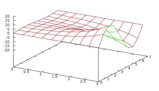
non uniform distributed vertices
A PDE of fourth order in four dimensions with non uniformly
distributed vertices of arbitrary geometry is difficult to
solve accurately. The building blocks are non uniform
four dimensional discretization, nuderiv4d.java.
The test program to check all 70 possible derivatives is
test_nuderiv4d.java.
A simple PDE
Uxxxx(x,y,z,t) + Uyyyy(x,y,z,t) + Uzzzz(x,y,z,t) + Utttt(x,y,z,t) =
2*(exp(x)+exp(y)+exp(z)+exp(t))
with solution
U(x,y,z,t) = exp(x)+exp(y)+exp(z)+exp(t)
is shown below.
It runs very fast, yet accuracy problems as number of unknown
vertices increases.
This is very sensitive to the independence of the underlying
grid points.
nuderiv4d.java basic discretization
test_nuderiv4d.java test discretization
pde44e_nuderiv4d.java PDE source code
pde44e_nuderiv4d_1_java.out PDE solution
A third degree PDE over the more linearly independent 4D grid points
shows the error degradation with more free vertices.
The output has three accuracy tests, for 1, 5 and 10 free nodes.
pde34_nuderiv4d.java PDE source code
pde34_nuderiv4d_1_java.out PDE solution
non uniform distributed vertices in Ada
Basically same code as above, in Ada
nuderiv4d.ads basic discretization spec
nuderiv4d.adb basic discretization body
test_nuderiv4d.adb test discretization
test_nuderiv4d_ada.out test discretization output
pde44e_nuderiv4d.adb PDE source code
pde44e_nuderiv4d_ada.out PDE solution, output
An extended example of discretization of a fourth order PDE in two
non uniform dimensions is shown in discrete2d.txt
Error increases with higher derivative and fewer points
The minimum number of points to compute a derivative of order n is n+1.
More points used decreases the error until numeric failure.
e.g. without multiple precision, third and fourth order derivative
fail with 11 points. An example of the variation of error from
computing the derivative on a sine wave is shown by
test_deriv.c source to test
deriv.c basic discretization, uniform spacing
test_deriv_c.out output showing test
Just general test, Python2 py and Python3 py3
deriv.py basic discretization, uniform spacing
test_deriv.py source to test
test_deriv_py.out output showing test
test_deriv.py3 source to test
test_deriv_py3.out output showing test
rderiv.py just deriv uniform spacing
test_rderiv.py source to test
test_rderiv_py.out output showing test
test_rderiv.py3 source to test
test_rderiv_py3.out output showing test
nuderiv.py just deriv, non uniform spacing
test_nuderiv.py source to test
test_nuderiv_py.out output showing test
More testing in ruby
Inverse.rb Inverse class
Deriv.rb Deriv class
test_deriv.prb source to test
test_deriv_rb.out output showing test
Non uniform discretization follows the same error pattern and the maximum
error goes approximately as the largest spacing between points.
Using Galerkin FEM on a fourth order Biharmonic PDE.
Two and three dimensions and parallel versions for C, Java, Ada and Python
Several versions of the Biharmonic PDE are used. First version is
∂4U(x,y)/∂x4 + 2 ∂4U(x,y)/∂x2∂y2 + ∂4U(x,y)/∂y4 +
2 ∂2U(x,y)/∂x2 + 2 ∂2U(x,y)/∂y2 + 2 U(x,y) = f(x,y)
First in two dimensions, then three dimensions.
Very few degrees of freedom are needed by using high order
shape functions and high order quadrature.
First, create test case with known solution.
Then, test that the test case is correctly coded in a language of your choice.
source code test_bihar2d.java
test output test_bihar2d.out
Plot after clicking "next" a few times.
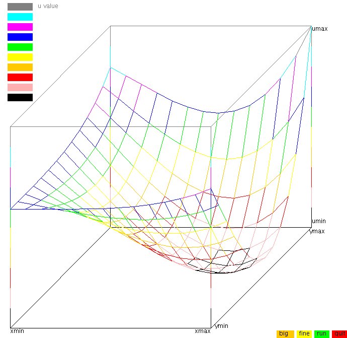 Next, include your test case in a PDE solver.
This case uses a previously covered Galerkin FEM with Lagrange shape functions.
Several choices higher order integration was used.
Several choices of degrees of freedom was used.
source code fem_bihar2d_la.java
output fem_bihar2d_la_java.out
source code fem_bihar2d_la.c
output fem_bihar2d_la_c.out
Plot of final solution, file plotted by gnuplot:
Next, include your test case in a PDE solver.
This case uses a previously covered Galerkin FEM with Lagrange shape functions.
Several choices higher order integration was used.
Several choices of degrees of freedom was used.
source code fem_bihar2d_la.java
output fem_bihar2d_la_java.out
source code fem_bihar2d_la.c
output fem_bihar2d_la_c.out
Plot of final solution, file plotted by gnuplot:
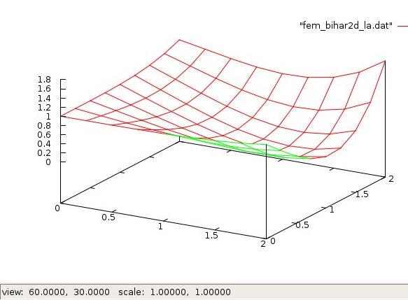
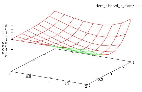 A multi language set of fourth order biharmonic PDE solutions.
High order shape function, high order quadrature, small DOF.
Wall time and checking solution against PDE included.
Expected solution is sin(x)*sin(y)
source code fem_bihar2dps_la.java
output fem_bihar2dps_la_java.out
source code fem_bihar2dps_la.c
output fem_bihar2dps_la_c.out
source code fem_bihar2dps_la.adb
output fem_bihar2dps_la_ada.out
source code fem_bihar2dps_la.f90
output fem_bihar2dps_la_f90.out
source code fem_bihar2dps_la.py
output fem_bihar2dps_la_py.out
A multi language set of fourth order biharmonic PDE solutions.
High order shape function, high order quadrature, small DOF.
Wall time and checking solution against PDE included.
Expected solution is sin(x)*sin(y)
source code fem_bihar2dps_la.java
output fem_bihar2dps_la_java.out
source code fem_bihar2dps_la.c
output fem_bihar2dps_la_c.out
source code fem_bihar2dps_la.adb
output fem_bihar2dps_la_ada.out
source code fem_bihar2dps_la.f90
output fem_bihar2dps_la_f90.out
source code fem_bihar2dps_la.py
output fem_bihar2dps_la_py.out
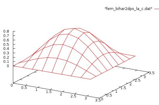
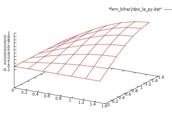
Now a three dimensional, fourth order Biharmonic PDE,
solved with few degrees of freedom and high order quadrature.
First, create test case with known solution.
Then, test that the test case is correctly coded in a language of your choice.
source code test_bihar3d.java
test output test_bihar3d.out
Plot after clicking "next" a few times.
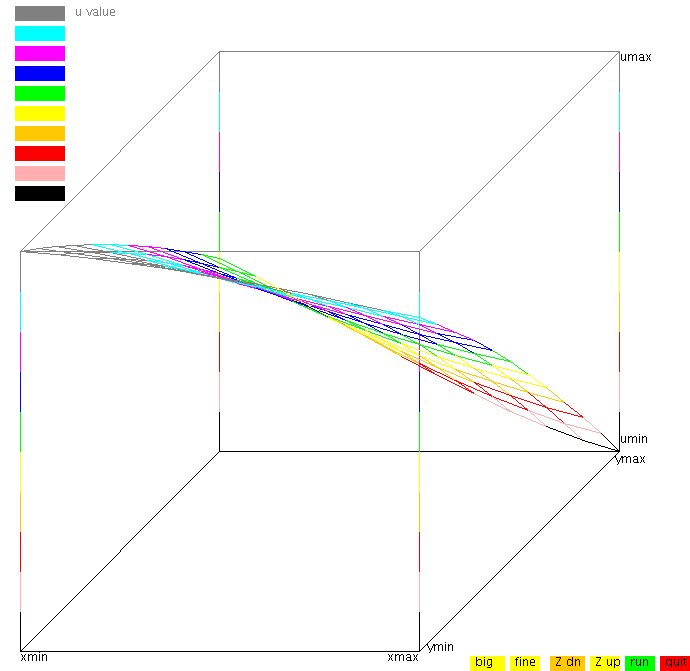 Next, include your test case in a PDE solver.
This case uses a previously covered Galerkin FEM with Lagrange shape functions.
Several choices higher order integration was used.
Several choices of degrees of freedom was used.
source code fem_bihar3d_la.java
output fem_bihar3d_la_java.out
source code fem_bihar3d_la.c
output fem_bihar3d_la_c.out
Plot of final solution at z=zmin, file plotted by gnuplot:
Next, include your test case in a PDE solver.
This case uses a previously covered Galerkin FEM with Lagrange shape functions.
Several choices higher order integration was used.
Several choices of degrees of freedom was used.
source code fem_bihar3d_la.java
output fem_bihar3d_la_java.out
source code fem_bihar3d_la.c
output fem_bihar3d_la_c.out
Plot of final solution at z=zmin, file plotted by gnuplot:
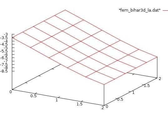
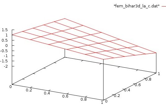
Using discretization on a fourth order Biharmonic PDE.
∂4U(x,y,z,t)/∂x4 + ∂4U(x,y,z,t)/∂y4 + ∂4U(x,y,z,t)/∂z4 + ∂4U(x,y,z,t)/∂t4 +
2 ∂2U(x,y,z,t)/∂x2 + 2 ∂2U(x,y,z,t)/∂y2 + 2 ∂2U(x,y,z,t)/∂z2 + 2 ∂2U(x,y,z,t)/∂t2 + 2 U(x,y,z,t) = f(x,y,z,t)
source code pde_bihar44t_eq.java
source code plot4d.java
output pde_bihar44t_eq_java.out
plot data pde_bihar44t_eq.dat
output plot4d.out
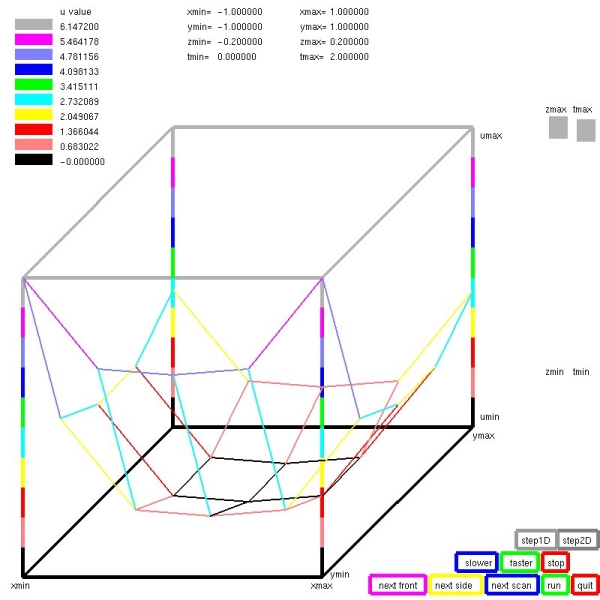 Three sets of boundary for homogeneous Biharmonic PDE four dimensions
show variation in accuracy of solution.
This code writes the solution to a file for plotting with plot4d_gl.
Ada source code pde44h_eq.adb
output pde44h_eq_ada.out
Three sets of boundary for homogeneous Biharmonic PDE four dimensions
show variation in accuracy of solution.
This code writes the solution to a file for plotting with plot4d_gl.
Ada source code pde44h_eq.adb
output pde44h_eq_ada.out
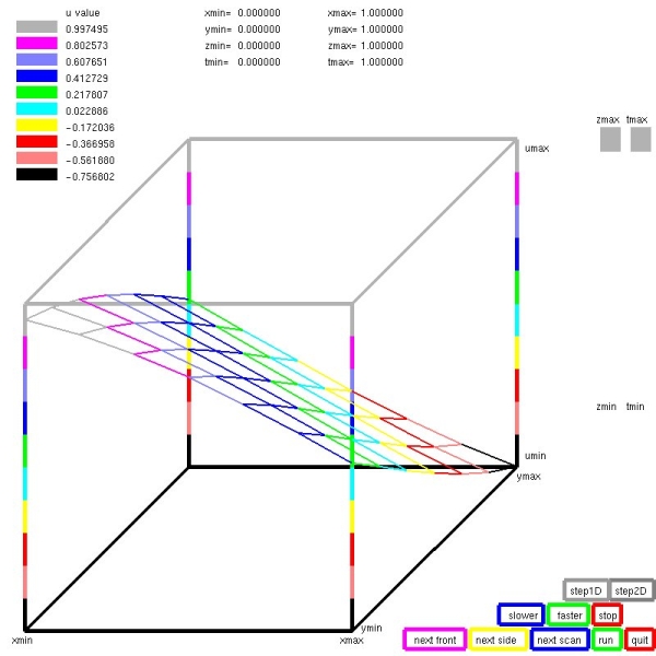 Other languages, homogeneous Biharmonic PDE in four dimensions
"C" source code pde44h_eq.c
output pde44h_eq_c.out
Fortran source code pde44h_eq.f90
output pde44h_eq_ada.f90
Java source code pde44h_eq.java
output pde44h_eq_java.out
Other languages, homogeneous Biharmonic PDE in four dimensions
"C" source code pde44h_eq.c
output pde44h_eq_c.out
Fortran source code pde44h_eq.f90
output pde44h_eq_ada.f90
Java source code pde44h_eq.java
output pde44h_eq_java.out
Now, make both the Java, C and Python code parallel, using threads,
Ada code parallel using tasks,
for a shared memory computer:
(coming soon for distributed memory)
source code femth_bihar2dps_la.java
output femth_bihar2dps_la_java.out
source code fempt_bihar2dps_la.c
output fempt_bihar2dps_la_c.out
source code femta_bihar2dps_la.adb
output femta_bihar2dps_la_ada.out
source code femth_bihar2dps_la.py
output femth_bihar2dps_la_py.out
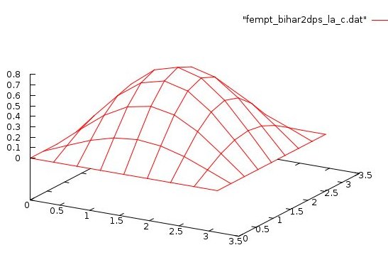 Other files, that are needed by some examples above:
Java
nderiv.java first to very high numerical derivatives
gaulegf.java low to very high order quadrature
simeq.java to about 10,000 DOF
laphi.java first through fourth order shape functions and derivatives
fem_bihar2dps_la.plot for gnuplot
femth_bihar2dps_la.plot for gnuplot
Ada
rderiv.adb first to very high numerical derivatives
deriv.adb derivative coefficients
test_deriv.adb code to check accuracy
test_deriv_ada.out accuracy limit 4th order, 11 points
gauleg.adb low to very high order quadrature
simeq.adb to about 10,000 DOF
laphi.ads first through fourth order shape functions and derivatives
laphi.adb body for above
real_arrays.ads real, real_vector, real_matrix
real_arrays.adb body for above
fem_bihar2dps_la_ada.plot for gnuplot
femta_bihar2dps_la_ada.plot for gnuplot
C
nderiv.c first to very high numerical derivatives
nderiv.h
gaulegf.c low to very high order quadrature
gaulegf.h
simeq.c to about 10,000 DOF
simeq.h
laphi.c first through fourth order shape functions and derivatives
laphi.h
fem_bihar2dps_la_c.plot for gnuplot
femth_bihar2dps_la_c.plot for gnuplot
Fortran
nderiv.f90 first to very high numerical derivatives
gaulegf.f90 low to very high order quadrature
simeq.f90 to about 10,000 DOF
laphi.f90 first through fourth order shape functions and derivatives
fem_bihar2dps_la_f90.plot for gnuplot
Python
deriv.py first to very high numerical derivatives
gauleg.py low to very high order quadrature
simeq.py to about 10,000 DOF
laphi.py first through fourth order shape functions and derivatives
pybarrier.py for parallel threads
fem_bihar2dps_la_py.plot for gnuplot
femth_bihar2dps_la_py.plot for gnuplot
Using discretization, more difficult to program, yet faster
Works for non uniform grid in both X and Y
pde_bihar2d_eq.java very fast
simeq.java very accurate for reasonable DOF
nuderiv.java very accurate for reasonable grid
pde_bihar2d_eq_java.out output
pde_bihar2d_eq.dat output data
pde_bihar2d_eq.plot plot
pde_bihar2d_eq.sh plot
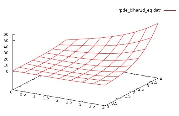 pde_bihar2d_eq.c very fast
simeq.c
nuderiv.c
pde_bihar2d_eq_c.out output
pde_bihar2d_eq_c.plot plot
pde_bihar2d_eq.c very fast
simeq.c
nuderiv.c
pde_bihar2d_eq_c.out output
pde_bihar2d_eq_c.plot plot
A difficult first order PDE in 4 dimensions
pde4sin_eq.adb
pde4sin_eq_ada.out
pde4sin_eq.dat
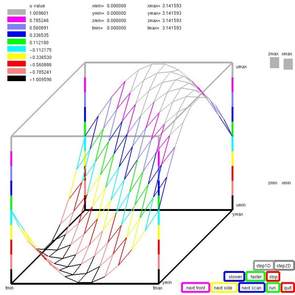
Another fourth order PDE
Kuramoto-Sivashinsky equation, is shown in Lecture 31b
More fourth order PDE
The Euler Bernoulli Beam Equation (static)
∂2w/∂x2 ( E I ∂2w/∂x2 ) = q
With EI constant
∂4w/∂x4 = q(x)
The Euler Lagrange Beam Equation (dynamic)
∂2w/∂x2 ( E I ∂2w/∂x2 ) = -μ ∂2w/∂t2 = q(x,t)
can be four independent variables w(x,y,x,t)
Many methods are needed for various PDE's
The Laplace Equation
∂2U/∂x2 + ∂2U/∂y2 = 0
Given the boundary conditions for 17 vertices in X and Y on
the unit square, using 17 points for derivatives, efficiently
solves U(x,y)=cos(k*x)*cosh(k*x) where k is about 2Pi.
Absolute error order 10E-5, with solution about -300 to 300
pde_laplace.c very fast
pde_laplace_c.out print output
pde_laplace_c.dat data output
pde_laplace_c.sh gnu plot
pde_laplace_c.plot plot
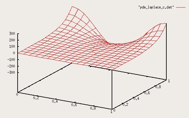
Another Laplace forth order, four dimension,
with parallel (thread) solution
This PDE needed 12th order discretization to obtain an
accuracy near 0.0001. Almost all of the execution time
was used solving 10,000 equations in 10,000 unknowns, DOF.
10 cores were used to keep the execution time to below
20 minutes rather than about 3 hours for a single core
execution.
∂4U(x,y,z,t)/∂x4 + ∂4U(x,y,z,t)/∂y4 + ∂4U(x,y,z,t)/∂z4 + ∂4U(x,y,z,t)/∂t4 +
2 ∂4U(x,y,z,t)/∂x2∂y2 + 2 ∂4U(x,y,z,t)/∂x2∂z2 +
2 ∂4U(x,y,z,t)/∂x2∂t2 + 2 ∂4U(x,y,z,t)/∂y2∂z2 +
2 ∂4U(x,y,z,t)/∂y2∂t2 + 2 ∂4U(x,y,z,t)/∂z2∂t2 -
16 U(x,y,z,t) = f(x,y,z,t) = 0
pde_bihar44tl_eq.c
pde_bihar44tl_eq_c.out
tsimeq.c
pde_bihar44tl_eq.adb
pde_bihar44tl_eq_ada.out
psimeq.adb
Plotted with plot4d_gl, one static view of the 4D solution is:
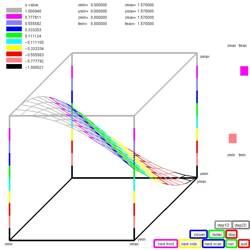
One version of Navier Stokes equation
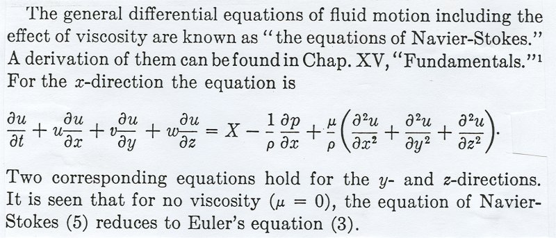
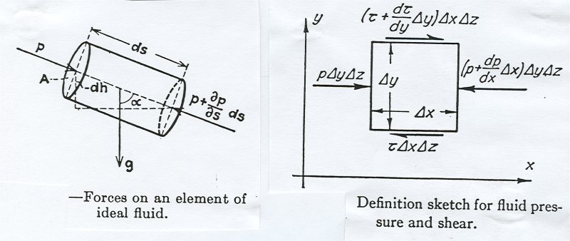
 Each term above has units of length over time squared, acceleration,
in meters per second squared. u is the three component velocity
vector, each component in meters per second, ρ is the fluid density
in kilograms per cubic meter, p is the pressure in newtons per square meter,
μ is the dynamic viscosity newton seconds per square meter.
X is externally applied acceleration, F/m, newtons per kilogram.
Another representation of Navier Stokes equation, multiplying the
above equation by ρ, yields terms that are force per unit volume,
newtons per cubic meter. del ∇ is the differential operator,
gradient. v is the velocity vector. b is externally applied acceleration.
Each term above has units of length over time squared, acceleration,
in meters per second squared. u is the three component velocity
vector, each component in meters per second, ρ is the fluid density
in kilograms per cubic meter, p is the pressure in newtons per square meter,
μ is the dynamic viscosity newton seconds per square meter.
X is externally applied acceleration, F/m, newtons per kilogram.
Another representation of Navier Stokes equation, multiplying the
above equation by ρ, yields terms that are force per unit volume,
newtons per cubic meter. del ∇ is the differential operator,
gradient. v is the velocity vector. b is externally applied acceleration.
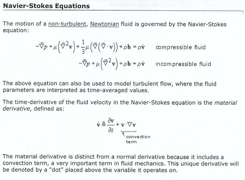 navier_gl.txt notes
navier_gl.c work in progress
navier_gl.out output attempt
navier_gl.txt notes
navier_gl.c work in progress
navier_gl.out output attempt
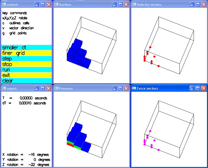 Some notes for your consideration:
1) You are expected to be intelligent enough to know the practical
limitations of equations that are given to you. When you develop
the equations, you must take into account practical limitations.
Many scholarly textbooks on differential equations make the
statement that a differential equation describing the physical
world is an approximation of what will actually happen. If you
keep stretching a spring using F = k x, the equation only
applies until the spring breaks.
2) We use the statement that "mass is conserved" in many physical
equations. Understand that the limits, usually unstated, are
"in a closed system and with no E = M C^2" Typically fluid equations
do not account for evaporation or fluid loss do to leaks or spillage.
The equations assume an absolutely closed system.
3) We use, as a fact "energy is conserved" in many physical equations.
Energy may take many forms and energy is easily converted from one
form to another and may not be taken into account by a specific equation.
For example, potential energy, a given mass at a given height, may
be released and potential energy is converted to kinetic energy.
Then, splat, the mass hits the ground in an inelastic collision and
has zero potential and zero kinetic energy. Most of the energy is
converted to heat energy with the possible conversion to some
chemical energy and some electrical energy.
Understand that heat and electrical energy can take the form
of radiation and leave what you are considering a "closed system."
4) Momentum is not conserved during a non elastic collision!
Fortunately, molecules of most fluids do not stick very often.
Surface tension must be taken into account when the fluid has
a surface open to the atmosphere. Capillary action affect must
be taken into account when a fluid "wets" a vertical surface.
5) When considering an infinitesimal volume, for example a cube in
a Cartesian measurement system. We generally take z to be the
vertical axis, meaning along a gravitational force line. We
consider a non compressible fluid in this cube with side s, to have
pressure applied to all six faces. Several cases are possible:
a) The fluid is stationary, what are the pressure on each face?
We define pressure as positive force divided by area into the cube.
aa) The cube of fluid has the same fluid on all sides.
Because of gravity, not all faces have the same pressure.
Given pressure P on the more positive X face, there must
be the same force P on the more negative X face else
the cube would accelerate and move. The pressure on both
Y faces must be the same P else fluid would move into or
out of the cube in the Y direction.
But, we are making an assumption that the pressure is constant
all over the X and Y faces yet this is an approximation. The
fluid has density and thus the mass is density times volume.
Mass is attracted by gravity. We can reasonably assume the force
of gravity does not change enough to be considered for the height
s, of our infinitesimal cube. Yet the pressure on the more positive
Z face must be considered different from the pressure on
the more negative Z face. Gravity puts a force of mass times
the gravitational constant g in the negative Z direction
on the fluid in the cube. With g taken as a constant, the
force is linear in the Z direction, thus the pressure P
on the X and Y faces is actually the pressure at the center
of each face. The pressure on the top, most positive Z face
is P - 1/2 rho * s * g and the pressure on the bottom,
most negative Z face is P + 1/2 rho * s * g. Pressure must
increase as depth increases.
ab) One or more face is against an immovable wall.
Same as aa)
b) The fluid is moving at a constant velocity.
ba) The cube of fluid has the same velocity as fluid on all sides.
Same as aa)
bb) The fluid against some face is moving at a different velocity.
Now we can not ignore viscosity. Viscosity is essentially a
measure of sliding resistance between the fluids at the faces
of two adjacent infinitesimal cubes.
c) The fluid is accelerating.
All of the above must be taken into account with the addition
of F = m a applied to the center of mass of the cube.
Consider the X direction with pressure P1 on the most negative
X face and a smaller P2 on the most positive X face. We can
apply the force (P1 - P2)*s^2 in the positive X direction to
the center of mass. Differences the pressure on Y faces are
independently applied to the Y direction. Use caution in
the Z direction, subtracting the difference in pressure due
to gravity because this does not impart an acceleration on
the center of mass when the infinitesimal cube has fluid or
an immovable surface under the cube.
It may be too late, but, don't panic, this was a small part of
Computational Fluid Dynamics, CFD. CFD is a large area and modeling
includes supersonic flight in complex scenarios.
More references:
navier_stokes.equation
navier_stokes_2d.equation
navier.equations breif
navier_fem.pdf technical paper
metric_units.txt metric definitions
also used in lecture 22 space satellite problem
air_prop.txt air properties
physics1.txt equations
convert_metric.pdf conversion
units.txt units definitions
Some notes for your consideration:
1) You are expected to be intelligent enough to know the practical
limitations of equations that are given to you. When you develop
the equations, you must take into account practical limitations.
Many scholarly textbooks on differential equations make the
statement that a differential equation describing the physical
world is an approximation of what will actually happen. If you
keep stretching a spring using F = k x, the equation only
applies until the spring breaks.
2) We use the statement that "mass is conserved" in many physical
equations. Understand that the limits, usually unstated, are
"in a closed system and with no E = M C^2" Typically fluid equations
do not account for evaporation or fluid loss do to leaks or spillage.
The equations assume an absolutely closed system.
3) We use, as a fact "energy is conserved" in many physical equations.
Energy may take many forms and energy is easily converted from one
form to another and may not be taken into account by a specific equation.
For example, potential energy, a given mass at a given height, may
be released and potential energy is converted to kinetic energy.
Then, splat, the mass hits the ground in an inelastic collision and
has zero potential and zero kinetic energy. Most of the energy is
converted to heat energy with the possible conversion to some
chemical energy and some electrical energy.
Understand that heat and electrical energy can take the form
of radiation and leave what you are considering a "closed system."
4) Momentum is not conserved during a non elastic collision!
Fortunately, molecules of most fluids do not stick very often.
Surface tension must be taken into account when the fluid has
a surface open to the atmosphere. Capillary action affect must
be taken into account when a fluid "wets" a vertical surface.
5) When considering an infinitesimal volume, for example a cube in
a Cartesian measurement system. We generally take z to be the
vertical axis, meaning along a gravitational force line. We
consider a non compressible fluid in this cube with side s, to have
pressure applied to all six faces. Several cases are possible:
a) The fluid is stationary, what are the pressure on each face?
We define pressure as positive force divided by area into the cube.
aa) The cube of fluid has the same fluid on all sides.
Because of gravity, not all faces have the same pressure.
Given pressure P on the more positive X face, there must
be the same force P on the more negative X face else
the cube would accelerate and move. The pressure on both
Y faces must be the same P else fluid would move into or
out of the cube in the Y direction.
But, we are making an assumption that the pressure is constant
all over the X and Y faces yet this is an approximation. The
fluid has density and thus the mass is density times volume.
Mass is attracted by gravity. We can reasonably assume the force
of gravity does not change enough to be considered for the height
s, of our infinitesimal cube. Yet the pressure on the more positive
Z face must be considered different from the pressure on
the more negative Z face. Gravity puts a force of mass times
the gravitational constant g in the negative Z direction
on the fluid in the cube. With g taken as a constant, the
force is linear in the Z direction, thus the pressure P
on the X and Y faces is actually the pressure at the center
of each face. The pressure on the top, most positive Z face
is P - 1/2 rho * s * g and the pressure on the bottom,
most negative Z face is P + 1/2 rho * s * g. Pressure must
increase as depth increases.
ab) One or more face is against an immovable wall.
Same as aa)
b) The fluid is moving at a constant velocity.
ba) The cube of fluid has the same velocity as fluid on all sides.
Same as aa)
bb) The fluid against some face is moving at a different velocity.
Now we can not ignore viscosity. Viscosity is essentially a
measure of sliding resistance between the fluids at the faces
of two adjacent infinitesimal cubes.
c) The fluid is accelerating.
All of the above must be taken into account with the addition
of F = m a applied to the center of mass of the cube.
Consider the X direction with pressure P1 on the most negative
X face and a smaller P2 on the most positive X face. We can
apply the force (P1 - P2)*s^2 in the positive X direction to
the center of mass. Differences the pressure on Y faces are
independently applied to the Y direction. Use caution in
the Z direction, subtracting the difference in pressure due
to gravity because this does not impart an acceleration on
the center of mass when the infinitesimal cube has fluid or
an immovable surface under the cube.
It may be too late, but, don't panic, this was a small part of
Computational Fluid Dynamics, CFD. CFD is a large area and modeling
includes supersonic flight in complex scenarios.
More references:
navier_stokes.equation
navier_stokes_2d.equation
navier.equations breif
navier_fem.pdf technical paper
metric_units.txt metric definitions
also used in lecture 22 space satellite problem
air_prop.txt air properties
physics1.txt equations
convert_metric.pdf conversion
units.txt units definitions
Just extending fourth order PDE in four dimensions, to five dimensions
Desired solution is U(w,x,y,z,t), given PDE:
.5 ∂4U(w,x,y,z,t)/∂w4 + 1.5 ∂4U(w,x,y,z,t)/∂w∂x∂y∂z + 2.5 ∂4U(w,x,y,z,t)/∂w2∂t2 +
∂4U(w,x,y,z,t)/∂x4 + 2 ∂4U(w,x,y,z,t)/∂y4 + 3 ∂4U(w,x,y,z,t)/∂z4 + 4 ∂4U(w,x,y,z,t)/∂t4 +
5 ∂3U(w,x,y,z,t)/∂x∂y∂t + 6 ∂4U(w,x,y,z,t)/∂y2∂z2 +
7 ∂3U(w,x,y,z,t)/∂z∂t2 + 8 ∂3U(w,x,y,z,t)/∂t3 + 9 ∂3U(w,x,y,z,t)/∂y2∂t +
10 ∂2U(w,x,y,z,t)/∂z∂t + 11 ∂U(w,x,y,z,t)/∂t + 12 U(w,x,y,z,t) = f(w,x,y,z,t)
With f(w,x,y,z,t) given in pde45.txt, Dirichlet boundary values from U(w,x,y,z,t)
Development requires test cases to verify correctness of code.
Check computing first through fourth order derivative of five variables:
test_5d.ads specification of test functions
test_5d.adb test functions
check_test_5d.adb check test functions
check_test_5d_ada.out check output
Now, test a fourth order PDE in five dimensions.
pde45_eq.adb extended pde44_eq.adb
pde45_eq_ada.out verification output
The test case used in pde45_eq was created with the help of Maple
pde45.txt text of Maple output
Plotting solution against 5D independent variables
Designed for interactive changing of variables plotted and variables values.
pot5d_gl.c plot program
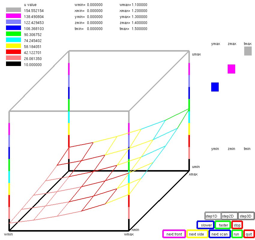
∇4U + 2 ∇2U + 5 U = 0
Fourth order Biharmonic PDE solution in 5 dimensions in "C"
pde45h_eq.c extended pde44h_eq.c
pde45h_eq_c.out output
Fourth order Biharmonic PDE solution in 5 dimensions in Fortran 90
pde45h_eq.f90 extended pde44h_eq.f90
pde45h_eq_f90.out output
Fourth order Biharmonic PDE solution in 5 dimensions in Java
pde45h_eq.java extended pde44h_eq.java
pde45h_eq_java.out output
Just extending fourth order PDE in four dimensions, to six dimensions
Desired solution is U(v,w,x,y,z,t), given PDE:
∇4U + 2 ∇2U + 6 U = 0
∂4U(v,w,x,y,z,t)/∂v4 + ∂4U(v,w,x,y,z,t)/∂w4 +
∂4U(v,w,x,y,z,t)/∂x4 + ∂4U(v,w,x,y,z,t)/∂y4 +
∂4U(v,w,x,y,z,t)/∂z4 + ∂4U(v,w,x,y,z,t)/∂t4 +
2 ∂2U(v,w,x,y,z,t)/∂v2 + 2 ∂2U(v,w,x,y,z,t)/∂w2 +
2 ∂2U(v,w,x,y,z,t)/∂x2 + 2 ∂2U(v,w,x,y,z,t)/∂y2 +
2 ∂2U(v,w,x,y,z,t)/∂z2 + 2 ∂2U(v,w,x,y,z,t)/∂t2 +
6 U(v,w,x,y,z,t) = 0
6D cubes and spheres
faces.c program
faces.out Data on 2D to 6D
test_faces.c program
test_faces.out sphere data
faces.java program
faces_java.out Data on 2D to 6D
test_faces.java program
test_faces_java.out sphere equations test
Test a fourth order PDE in six dimensions.
∇4U + 2 ∇2U + 6 U = 0
pde46h_eq.adb extended pde44h_eq.adb
pde46h_eq_ada.out verification output
∇4U + 2 ∇2U + 6 U = 0
pde46h_eq.c
pde46h_eq_c.out verification output
∇4U + 2 ∇2U + 6 U = 0
pde46h_eq.f90
pde46h_eq_f90.out verification output
∇4U + 2 ∇2U + 6 U = 0
pde46h_eq.java
pde46h_eq_java.out verification output
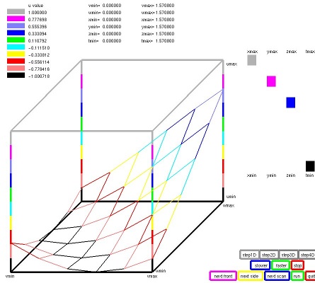 Plotted with plot6d_gl.c, stopped on one of the moving output
pde46h_eq_java.dat data written for plot
∇4P + 2 ∇2P = f(x,y,z,t,u,v)
Solving for P = exp(x+y+t*z+u+v) six independent variables, 4th order
pde64eb_eq.c testing source code
pde64eb_eq_c.out verification output
d6p4eb.mw Maple test generation
∇4P + 2 ∇2P = f(x,y,z,t,u,v)
Solving for P = sin(x*u+y*v+z+t) six independent variables, 4th order
pde64sb_eq.c testing source code
pde64sb_eq_c.out verification output
d6p4sb.mw Maple test generation
d6p4sb_rhs.jpg RHS
Plotted with plot6d_gl.c, stopped on one of the moving output
pde46h_eq_java.dat data written for plot
∇4P + 2 ∇2P = f(x,y,z,t,u,v)
Solving for P = exp(x+y+t*z+u+v) six independent variables, 4th order
pde64eb_eq.c testing source code
pde64eb_eq_c.out verification output
d6p4eb.mw Maple test generation
∇4P + 2 ∇2P = f(x,y,z,t,u,v)
Solving for P = sin(x*u+y*v+z+t) six independent variables, 4th order
pde64sb_eq.c testing source code
pde64sb_eq_c.out verification output
d6p4sb.mw Maple test generation
d6p4sb_rhs.jpg RHS
Plotting solution against 6D independent variables
Designed for interactive changing of variables plotted and variables values.
pot6d_gl.c plot program
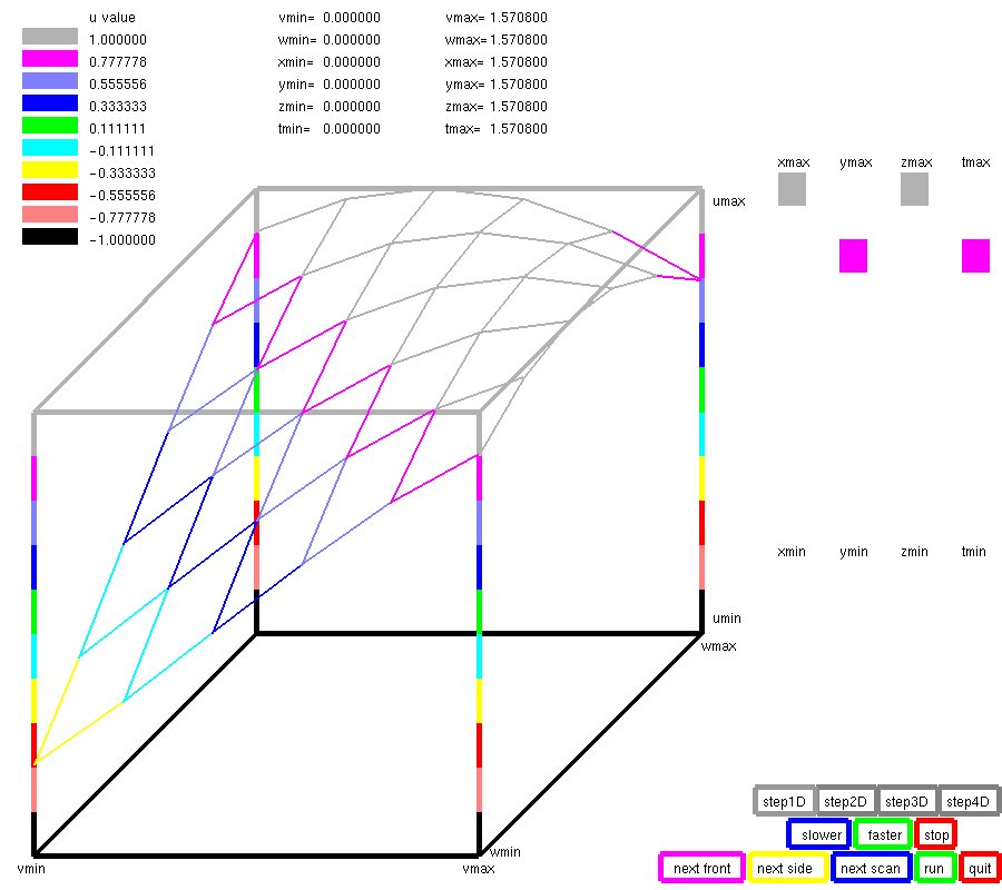
With a small change, we obtain a nonuniform refinement
Now we use "nuderiv" rather than "rderiv" that can use
nonuniform and different grids in each dimension.
Test a fourth order PDE in six dimensions with nonuniform refinement.
∇4U + 2 ∇2U + 6 U = 0
pde46h_nu.adb extended pde46h_eq.adb
pde46h_nu_ada.out verification output
∇4U + 2 ∇2U + 6 U = 0
pde46h_nu.java
pde46h_nu_java.out verification output
∇4U + 2 ∇2U + 6 U = 0
pde46h_nu.c
pde46h_nu_c.out verification output
Plotting solution against 6D independent variables
Designed for interactive changing of variables plotted and variables values.
pot6d_gl.c plot program
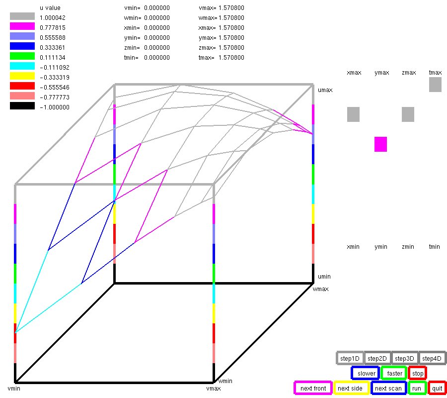 pde46h_nu_ada.jpg
Least Square Fit 6 independent variables up to sixth power
lsfit.ads Least Square Fit 6D 6P
lsfit.adb Least Square Fit 6D 6P
test_lsfit6.adb test program
test_lsfit6_ada.out test results
Some programs above also need
simeq.f90 solve simultaneous equations
deriv.f90 compute numerical derivatives
array3d.ads 3D arrays
array4d.ads 4D arrays
array5d.ads 5D arrays
array6d.ads 6D arrays
real_arrays.ads 2D arrays and operations
real_arrays.adb 2D arrays and operations
integer_arrays.ads 2D arrays and operations
integer_arrays.adb 2D arrays and operations
You won't find many free or commercial 5D and 6D PDE packages
many lesser problems have many opensource and commercial packages
en.wikipedia.org/wiki/list_of_finite_element_software_packages
Just extending fourth order PDE in four dimensions, to seven dimensions
Desired solution is U(x,y,z,t,u,v,w), given PDE:
∇4U + 2 ∇2U + 8 U = f(x,y,z,t,u,v,w)
∂4U(x,y,z,t,u,v,w)/∂x4 + ∂4U(x,y,z,t,u,v,w)/∂y4 +
∂4U(x,y,z,t,u,v,w)/∂z4 + ∂4U(x,y,z,t,u,v,w)/∂t4 +
∂4U(x,y,z,t,u,v,w)/∂u4 + ∂4U(x,y,z,t,u,v,w)/∂v4 +
∂4U(x,y,z,t,u,v,w)/∂w4 +
2 ∂2U(x,y,z,t,u,v,w)/∂x2 + 2 ∂2U(x,y,z,t,u,v,w)/∂y2 +
2 ∂2U(x,y,z,t,u,v,w)/∂z2 + 2 ∂2U(x,y,z,t,u,v,w)/∂t2 +
2 ∂2U(x,y,z,t,u,v,w)/∂u2 + 2 ∂2U(x,y,z,t,u,v,w)/∂v2 +
2 ∂2U(x,y,z,t,u,v,w)/∂w2 +
8 U(x,y,z,t,u,v,w) = f(x,y,z,t,u,v,w)
Test a fourth order PDE in seven dimensions.
∇4U + 2 ∇2U + 8 U = f(x,y,z,t,u,v,w)
pde47h_nu.adb extended pde46h_nu.adb
pde47h_nu_ada.out verification output
pde47h_eq.adb solver source code
pde47h_eq_ada.out verification output
pde47h_eq.f90 solver source code
pde47h_eq_f90.out verification output
Test a fourth order PDE in seven dimensions.
∇4U + 2 ∇2U + 8 U = f(x,y,z,t,u,v,w)
pde47h_nu.java extended pde46h_nu.java
pde47h_nu_java.out verification output
pde47h_eq.java solver source code
pde47h_eq_java.out verification output
with i7, j7 in place of iiiiiii, jjjjjjj
pde47hn_eq.java solver source code
pde47hn_eq_java.out verification output
∇4U + 2 ∇2U + 8 U = f(x,y,z,t,u,v,w)
pde47h_nu.c
pde47h_nu_c.out verification output
pde47h_eq.c solver source code
pde47h_eq_c.out verification output
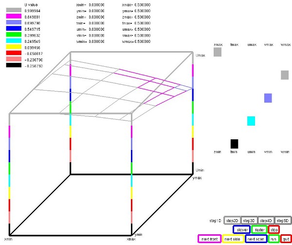 Plotted with plot7d_gl.c, stopped on one of the moving output
pde47h_nu_c1.dat data written for plot
Plotted with plot7d_gl.c, stopped on one of the moving output
pde47h_nu_c1.dat data written for plot
Boltzmann Equation in seven dimensions, using Galerkin FEM.
∇U(x,y,z,t,p,q,r) = Sf(x,y,z,t,p,q,r)
boltzmann_7la.java extended fem_check44_la.java
boltzmann_7la_java.out verification output
boltzmann_7la.dat for plot7d_gl and lsfit_file
least square fit of 7 dimensional data
lsfit.adb Least square fit, up to 7 dimensions, 4th order
test_lsfit7.adb Test least square fit, up to 7 dimensions, 4th order
test_lsfit7_ada.out Test results
lsfit.java Least square fit, up to 7 dimensions, 4th order
lsfit_file.java fit polynomial solution to PDE numerical solution
lsfit_file_java7.out Test results
Some programs above also need:
simeq.f90 solver
deriv.f90 numerical derivatives
array3d.ads 3D arrays
array4d.ads 4D arrays
array5d.ads 5D arrays
array6d.ads 6D arrays
array7d.ads 7D arrays
real_arrays.ads 2D arrays and operations
real_arrays.adb 2D arrays and operations
integer_arrays.ads 2D arrays and operations
integer_arrays.adb 2D arrays and operations
nuderiv.java basic non uniform grid derivative
rderiv.java basic uniform grid derivative
simeq.java basic simultaneous equation
deriv.h basic derivatives
deriv.c basic derivatives
plot7d_gl.c plot solution to PDE
You won't find many open source or commercial 7D PDE packages
many lesser problems have many open source and commercial packages
en.wikipedia.org/wiki/list_of_finite_element_software_packages
Just extending seventh order PDE in four dimensions, to eight dimensions
Desired solution is U(x,y,z,t,u,v,w,p), given PDE:
∇4U + 2 ∇2U + 8 U = f(x,y,z,t,u,v,w,p)
∂4U(x,y,z,t,u,v,w,p)/∂x4 + ∂4U(x,y,z,t,u,v,w,p)/∂y4 +
∂4U(x,y,z,t,u,v,w,p)/∂z4 + ∂4U(x,y,z,t,u,v,w,p)/∂t4 +
∂4U(x,y,z,t,u,v,w,p)/∂u4 + ∂4U(x,y,z,t,u,v,w,p)/∂v4 +
∂4U(x,y,z,t,u,v,w,p)/∂w4 + ∂4U(x,y,z,t,u,v,w,p)/∂p4 +
2 ∂2U(x,y,z,t,u,v,w,p)/∂x2 + 2 ∂2U(x,y,z,t,u,v,w,p)/∂y2 +
2 ∂2U(x,y,z,t,u,v,w,p)/∂z2 + 2 ∂2U(x,y,z,t,u,v,w,p)/∂t2 +
2 ∂2U(x,y,z,t,u,v,w,p)/∂u2 + 2 ∂2U(x,y,z,t,u,v,w,p)/∂v2 +
2 ∂2U(x,y,z,t,u,v,w,p)/∂w2 + 2 ∂2U(x,y,z,t,u,v,w,p)/∂p2 +
8 U(x,y,z,t,u,v,w,p) = f(x,y,z,t,u,v,w,p)
Test a fourth order PDE in eight dimensions.
∇4U + 2 ∇2U + 8 U = f(x,y,z,t,u,v,w,p)
pde48hn_eq.java solver source code
pde48hn_eq_java.out verification output
∇4U + 2 ∇2U + 8 U = f(x,y,z,t,u,v,w,p)
pde48hn_eq.c solver source code
pde48hn_eq_c.out verification output
pde48hn_eq.adb solver source code
pde48hn_eq_ada.out verification output
pde48h_eq.adb solver source code
pde48h_eq_ada.out verification output
Some programs above also need:
nuderiv.java basic non uniform grid derivative
rderiv.java basic uniform grid derivative
simeq.java basic simultaneous equation
deriv.h basic derivatives
deriv.c basic derivatives
real_arrays.ads 2D arrays and operations
real_arrays.adb 2D arrays and operations
integer_arrays.ads 2D arrays and operations
integer_arrays.adb 2D arrays and operations
rderiv.adb derivative computation
inverse.adb inverse computation
Plotted output from pde48hn_eq.java execution
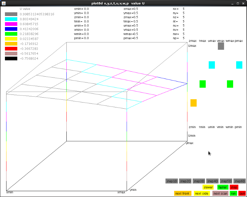 plot8d.java source code
User can select any two variables for 3D view.
User can select values for other variables, option to run all cases.
Then, going to a spherical coordinate system in 8 dimensions
gen_8d_sphere.c source equations
gen_8d_sphere_c.out verification output
plot8d.java source code
User can select any two variables for 3D view.
User can select values for other variables, option to run all cases.
Then, going to a spherical coordinate system in 8 dimensions
gen_8d_sphere.c source equations
gen_8d_sphere_c.out verification output
The above was all Cartesian Coordinates, now Spherical Coordinates
faces.c source code for output
faces.out output for n dimensional cube and spheretest_faces.c source code for test
test_faces.out output of test
faces.java source code for output
faces_java.out output for n dimensional cube and sphere
test_faces.java source code for test
test_faces_java.out equations and test
faces.py source code for output
faces_py.out output for n dimensional cube and sphere
faces.java running, data for various n-cubes, n-spheres, n dimensions
edge length L for cubes, radius R for spheres
0-cube point
vertices = 1
n=1-cube line
edges = 1 length=L
vertices = 2
n=2-cube square
2D faces = 1 area= L^2
edges = 4 length=4*L
vertices = 4
n=3-cube cube
cubes = 1 volume= L^3
2D faces = 6 area= 6*L^2
edges = 12 length=12*L
vertices = 8
n=4-cube
4-cubes = 1 volume= L^4
cubes = 8 volume= 8*L^3
2D faces = 24 area= 24*L^2
edges = 32 length=32*L
vertices = 16
n=5-cube
5-cubes = 1 volume= L^5
4-cubes = 10 volume=10*L^4
cubes = 40 volume=40*L^3
2D faces = 80 area= 80*L^2
edges = 80 length=80*L
vertices = 32
n=6-cube
6-cubes = 1 volume= L^6
5-cubes = 12 volume= 12*L^5
4-cubes = 60 volume= 60*L^4
cubes = 160 volume=160*L^3
2D faces = 240 area= 240*L^2
edges = 192 length=192*L
vertices = 64
n=7-cube
7-cubes = 1 volume= L^7
6-cubes = 14 volume= 14*L^6
5-cubes = 84 volume= 84*L^5
4-cubes = 280 volume=280*L^4
cubes = 560 volume=560*L^3
2D faces = 672 area= 672*L^2
edges = 448 length=448*L
vertices = 128
n=8-cube
8-cubes = 1 volume= L^8
7-cubes = 16 volume= 16*L^7
6-cubes = 112 volume= 112*L^6
5-cubes = 448 volume= 448*L^5
4-cubes = 1120 volume=1120*L^4
cubes = 1792 volume=17928L^3
2D faces = 1792 area= 1792*L^2
edges = 1024 length=1024*L
vertices = 256
n=9-cube
9-cubes = 1 volume= L^9
8-cubes = 18 volume= 18*L^8
7-cubes = 144 volume= 144*L^7
6-cubes = 672 volume= 672*L^6
5-cubes = 2016 volume=2016*L^5
4-cubes = 4032 volume=4032*L^4
cubes = 5376 volume=5376*L^3
2D faces = 4608 area= 4608*L^2
edges = 2304 length=2304*L
vertices = 512
n=10-cube
10-cubes = 1 volume= L^10
9-cubes = 20 volume= 20*L^9
8-cubes = 180 volume= 180*L^8
7-cubes = 960 volume= 960*L^7
6-cubes = 3360 volume= 3360*L^6
5-cubes = 8064 volume= 8064*L^5
4-cubes = 13440 volume=13440*L^4
cubes = 15360 volume=15360*L^3
2D faces = 11520 area= 11520*L^2
edges = 5120 length= 5120*L
vertices = 1024
cubes of n dimensions
with edge length E, n>=3, volume = E^n, area=(2D faces)*E*E
n-cube has 2^n vertex, with n edges at each vertex
n>=m, there are pwr2(n-m)*comb(n,m) n-m sub cubes
Spheres up to 10 dimensions
D-1 surface D volume
2D circle 2 Pi R 1 Pi R^2
3D sphere 4 Pi R^2 4/3 Pi R^3
4D 4-sphere 2 Pi^2 R^3 1/2 Pi^2 R^4
5D 5-sphere 8/3 Pi^2 R^4 8/15 Pi^2 R^5
6D 6-sphere 1 Pi^3 R^5 1/6 Pi^3 R^6
7D 7-sphere 16/15 Pi^3 R^6 16/105 Pi^3 R^7
8D 8-sphere 1/3 Pi^4 R^7 1/24 Pi^4 R^8
9D 9-sphere 32/105 Pi^4 R^8 32/945 Pi^4 R^9
10D 10-sphere 1/12 Pi^5 R^9 1/120 Pi^5 R^10
volume V_n(R)= Pi^(n/2) R^n / gamma(n/2+1)
gamma(integer) = factorial(integer-1) gamma(5) = 24
gamma(1/2) = sqrt(Pi), gamma(n/2+1) = (2n)! sqrt(Pi)/(4^n n!)
or V_2k(R) = Pi^k R^2k/k! , V_2k+1 = 2 k! (4Pi)^k R^(2k+1)/(2k+1)!
surface area A_n(R) = d/dR V_n(R)
one definition of sequence of n-spheres
a1, a2, a3, a4, a5, a6, a7 are angles, typ: theta, phi, ...
x1, x2, x3, x4, x5, x6, x7, x8 are orthogonal coordinates
x1^2 + x2^2 + x3^2 + x4^2 + x5^2 + x6^2 + x7^2 +x8^2 = R^2
Radius R = sqrt(R^2)
2D circle
x1 = R cos(a1) typ: x theta
x2 = R sin(a1) typ: y theta
a1 = arctan(x2/x1) or a1 = acos(x1/R)
3D sphere
x1 = R cos(a1) typ: z phi
x2 = R sin(a1) cos(a2) typ: x phi theta
x3 = R sin(a1) sin(a2) typ: y phi theta
a1 = arctan(sqrt(x2^2+x3^2)/x1) or a1 = acos(x1/R)
a2 = arctan(x3/x2) or a2 = acos(x2/sqrt(x2^2+x3^2))
4D 4-sphere continuing systematic notation, notice pattern
x1 = R cos(a1)
x2 = R sin(a1) cos(a2)
x3 = R sin(a1) sin(a2) cos(a3)
x4 = R sin(a1) sin(a2) sin(a3)
a1 = acos(x1/sqrt(x1^2+x2^2+x3^2+x4^2))
a2 = acos(x2/sqrt(x2^2+x3^2+x4^2))
a3 = acos(x3/sqrt(x3^2+x4^2)) if x4>=0
a3 = 2 Pi - acos(x3/sqrt(x3^2+x4^2)) if x4<0
5D 5-sphere
x1 = R cos(a1)
x2 = R sin(a1) cos(a2)
x3 = R sin(a1) sin(a2) cos(a3)
x4 = R sin(a1) sin(a2) sin(a3) cos(a4)
x5 = R sin(a1) sin(a2) sin(a3) sin(a4)
a1 = acos(x1/sqrt(x1^2+x2^2+x3^2+x4^2+x5^2))
a2 = acos(x2/sqrt(x2^2+x3^2+x4^2+x5^2))
a3 = acos(x3/sqrt(x3^2+x4^2+x5^2))
a4 = acos(x4/sqrt(x4^2+x5^2)) if x5>=0
a4 = 2 Pi - acos(x4/sqrt(x4^2+x5^2)) if x5<0
6D 6-sphere
x1 = R cos(a1)
x2 = R sin(a1) cos(a2)
x3 = R sin(a1) sin(a2) cos(a3)
x4 = R sin(a1) sin(a2) sin(a3) cos(a4)
x5 = R sin(a1) sin(a2) sin(a3) sin(a4) cos(a5)
x6 = R sin(a1) sin(a2) sin(a3) sin(a4) sin(a5)
a1 = acos(x1/sqrt(x1^2+x2^2+x3^2+x4^2+x5^2+x6^2))
a2 = acos(x2/sqrt(x2^2+x3^2+x4^2+x5^2+x6^2))
a3 = acos(x3/sqrt(x3^2+x4^2+x5^2+x6^2))
a4 = acos(x4/sqrt(x4^2+x5^2+x6^2))
a5 = acos(x5/sqrt(x5^2+x6^2)) if x6>=0
a5 = 2 Pi - acos(x5/sqrt(x5^2+x6^2)) if x6<0
7D 7-sphere
x1 = R cos(a1)
x2 = R sin(a1) cos(a2)
x3 = R sin(a1) sin(a2) cos(a3)
x4 = R sin(a1) sin(a2) sin(a3) cos(a4)
x5 = R sin(a1) sin(a2) sin(a3) sin(a4) cos(a5)
x6 = R sin(a1) sin(a2) sin(a3) sin(a4) sin(a5) cos(a6)
x7 = R sin(a1) sin(a2) sin(a3) sin(a4) sin(a5) sin(a6)
a1 = acos(x1/sqrt(x1^2+x2^2+x3^2+x4^2+x5^2+x6^2+x7^2))
a2 = acos(x2/sqrt(x2^2+x3^2+x4^2+x5^2+x6^2+x7^2))
a3 = acos(x3/sqrt(x3^2+x4^2+x5^2+x6^2+x7^2))
a4 = acos(x4/sqrt(x4^2+x5^2+x6^2+x7^2))
a5 = acos(x5/sqrt(x5^2+x6^2+x7^2))
a6 = acos(x6/sqrt(x6^2+x6^2)) if x7>=0
a6 = 2 Pi - acos(x6/sqrt(x6^2+x7^2)) if x7<0
8D 8-sphere
x1 = R cos(a1)
x2 = R sin(a1) cos(a2)
x3 = R sin(a1) sin(a2) cos(a3)
x4 = R sin(a1) sin(a2) sin(a3) cos(a4)
x5 = R sin(a1) sin(a2) sin(a3) sin(a4) cos(a5)
x6 = R sin(a1) sin(a2) sin(a3) sin(a4) sin(a5) cos(a6)
x7 = R sin(a1) sin(a2) sin(a3) sin(a4) sin(a5) sin(a6) cos(a7)
x8 = R sin(a1) sin(a2) sin(a3) sin(a4) sin(a5) sin(a6) sin(a7)
a1 = acos(x1/sqrt(x1^2+x2^2+x3^2+x4^2+x5^2+x6^2+x7^2+x8^2))
a2 = acos(x2/sqrt(x2^2+x3^2+x4^2+x5^2+x6^2+x7^2+x8^2))
a3 = acos(x3/sqrt(x3^2+x4^2+x5^2+x6^2+x7^2+x8^2))
a4 = acos(x4/sqrt(x4^2+x5^2+x6^2+x7^2+x8^2))
a5 = acos(x5/sqrt(x5^2+x6^2+x7^2+x8^2))
a6 = acos(x6/sqrt(x5^2+x6^2+x7^2+x8^2))
a7 = acos(x7/sqrt(x7^2+x8^2)) if x8>=0
a7 = 2 Pi - acos(x7/sqrt(x7^2+x8^2)) if x8<0
faces.java finished
It is left as an exercise to student to develop equations
for gradient and laplacian 4D to 8D spheres.
You won't find many open source or commercial 8D PDE packages
many lesser problems have many open source and commercial packages
en.wikipedia.org/wiki/list_of_finite_element_software_packages
Just extending eighth order PDE in four dimensions, to nine dimensions
Desired solution is U(x,y,z,t,u,v,w,p,q), given PDE:
∇4U + 2 ∇2U + 10 U = f(x,y,z,t,u,v,w,p,q)
∂4U(x,y,z,t,u,v,w,p,q)/∂x4 + ∂4U(x,y,z,t,u,v,w,p,q)/∂y4 +
∂4U(x,y,z,t,u,v,w,p,q)/∂z4 + ∂4U(x,y,z,t,u,v,w,p,q)/∂t4 +
∂4U(x,y,z,t,u,v,w,p,q)/∂u4 + ∂4U(x,y,z,t,u,v,w,p,q)/∂v4 +
∂4U(x,y,z,t,u,v,w,p,q)/∂w4 + ∂4U(x,y,z,t,u,v,w,p,q)/∂p4 +
∂4U(x,y,z,t,u,v,w,p,q)/∂q4 +
2 ∂2U(x,y,z,t,u,v,w,p,q)/∂x2 + 2 ∂2U(x,y,z,t,u,v,w,p,q)/∂y2 +
2 ∂2U(x,y,z,t,u,v,w,p,q)/∂z2 + 2 ∂2U(x,y,z,t,u,v,w,p,q)/∂t2 +
2 ∂2U(x,y,z,t,u,v,w,p,q)/∂u2 + 2 ∂2U(x,y,z,t,u,v,w,p,q)/∂v2 +
2 ∂2U(x,y,z,t,u,v,w,p,q)/∂w2 + 2 ∂2U(x,y,z,t,u,v,w,p,q)/∂p2 +
2 ∂2U(x,y,z,t,u,v,w,p,q)/∂q2 +
10 U(x,y,z,t,u,v,w,p,q) = f(x,y,z,t,u,v,w,p,q)
Maple check on solution
pde49hn_mws.out analytic solution
Test a fourth order PDE in nine dimensions.
∇4U + 2 ∇2U + 10 U = f(x,y,z,t,u,v,w,p,q)
pde49hn_eq.c solver source code
pde49hn_eq_c.out verification output
pde49h_eq.adb solver source code
pde49h_eq_ada.out verification output
pde49hn_eq.java solver source code
pde49hn_eq_java.out verification output
Some programs above also need:
nuderiv.java basic non uniform grid derivative
rderiv.java basic uniform grid derivative
simeq.java basic simultaneous equation
deriv.h basic derivatives
deriv.c basic derivatives
real_arrays.ads 2D arrays and operations
real_arrays.adb 2D arrays and operations
integer_arrays.ads 2D arrays and operations
integer_arrays.adb 2D arrays and operations
Plotted output from pde49hn_eq.c execution
plot9d.java plotter source code
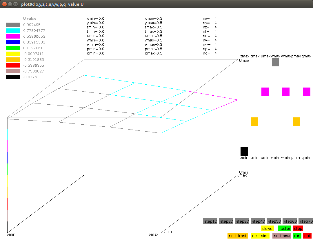 User can select any two variables for 3D view.
User can select values for other variables, option to run all cases.
User can select any two variables for 3D view.
User can select values for other variables, option to run all cases.
You won't find many open source or commercial 9D PDE packages
many lesser problems have many open source and commercial packages
en.wikipedia.org/wiki/list_of_finite_element_software_packages
Extending PDE's in polar, cylindrical, spherical
solve PDE in polar coordinates
∇2U(r,Θ) + U(r,Θ) = f(r,Θ)
given Dirichlet boundary values and f
Development version with much checking:
pde_polar_eq.adb
pde_polar_eq_ada.out
solve PDE in cylindrical coordinates
∇2U(r,Θ,z) + U(r,Θ,z) = f(r,Θ,z)
given Dirichlet boundary values and f
reference equations, cylindrical, spherical
Theta and Phi reversed from my programs.
Del_in_cylindrical_and_spherical_coordinates
Development version with much checking:
check_cylinder_deriv.c
check_cylinder_deriv_c.out
pde_cylinderical_eq.c
pde_cylinderical_eq_c.out
check_cylinder_deriv.java
check_cylinder_deriv_java.out
pde_cylinderical_eq.java
pde_cylinderical_eq_java.out
check_cylinder_deriv.adb
check_cylinder_deriv_ada.out
pde_cylinderical_eq.adb
pde_cylinderical_eq_ada.out
solve PDE in spherical coordinates
∇2U(r,Θ,Φ) + U(r,Θ,Φ) = f(r,Θ,Φ)
given Dirichlet boundary values and f
Development versions with much checking:
check_sphere_deriv.c
check_sphere_deriv_c.out
pde_spherical_eq.c
pde_spherical_eq_c.out
check_sphere_deriv.java
check_sphere_deriv_java.out
check_sphere_deriv.adb
check_sphere_deriv_ada.out
check_sphere_deriv.adb
check_sphere_deriv_ada.out
pde_spherical_eq.adb
pde_spherical_eq_ada.out
pde_spherical_eq.f90
pde_spherical_eq_f90.out
Another set using spherical laplacian
spherical_deriv.java
spherical_deriv_java.out
spherical_pde.mws Maple input
spherical_pde_mws.out Maple output
spherical_deriv.sh gnuplot
spherical_deriv.plot gnuplot
spherical_deriv.dat gnuplot data
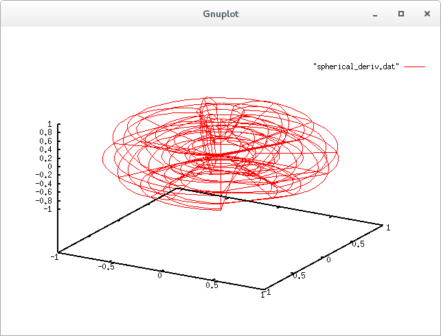 Other utility files needed by sample code above:
simeq.h
simeq.c
nuderiv.h
nuderiv.c
simeq.java
nuderiv.java
simeqb.adb
nuderiv.adb
nuderiv.f90
inverse.f90
May be converted to other languages.
Also possible, other toroidal coordinates.
Other utility files needed by sample code above:
simeq.h
simeq.c
nuderiv.h
nuderiv.c
simeq.java
nuderiv.java
simeqb.adb
nuderiv.adb
nuderiv.f90
inverse.f90
May be converted to other languages.
Also possible, other toroidal coordinates.
Spherical Laplacian in higher dimensions, 4 and 8 tested
// nabla.c del^2 = nabla = Laplacian n dimensional space of function U(r,a)
// n-dimensional sphere, radius r
// a[0],...,a[n-2] are angles in radians (User can rename in their code)
// compute Laplacian of U(r,a) at given angles
// double nabla(int n, double r, double a[], double (*U()));
//
// alternate call if partial derivative values of U are known
// da[0],...,da[n-2] are first partial derivatives of users U(r,a)
// dda[0],...,dda[n-2] are second partial derivatives of users U(r,a)
// with respect to a[0],...,a[n-2] evaluated
// at a[0],...,a[n-1]
// double nablapd(int n, double r, double a[],
// double dr, double ddr, double da[], double dda[]);
//
// utility function for n-dimensional cartesian to spherical coordinates
// n>3 x[0..n-1] r, a[0..n-2]
// void toSpherical(int n, double x[], double *r, double a[]);
//
// utility function for n-dimensional spherical to cartesian coordinates
// n>3 r, a[0..n-2] x[0..n-1]
// void toCartesian(int n, double r, double a[], double x[]);
//
// utility function for n-dimensional U(r, a) at r, a[]
// to derivatives da[] and dda[]
// void sphereDeriv(int n, double (*U)(), double r, double a[],
// double *dr, double *drr, double da[], double dda[]);
//
// method for basic nabla_n:
// use iterative function, n>3, for computing nabla_n of U(r,a[])
// using d for partial derivative symbol and U for U(r,a[]) and
// adjusting subscripts for a[0],...,a[n-2]
//
// before reduction for numerical computation:
// nabla_n = 1/r^n-1 d(r^n-1 dU/dr)/dr + 1/r^2 L2(n)
//
// after reduction:
// nabla_n = (n-1)/r dU/dr + d^2U/dr^2 + 1/r^2 L2(n, r, a)
//
// in code:
// nabla_n = ((n-1)/r)*dr + ddr + (1.0/(r*r))*L2(n,r,a);
//
// before reduction and adjusting subscripts of a_i code a[]:
// L2(n,r,a) = sum(i=2,n){prod(j=i+1,n){1/sin^2(a_j)} *
// 1/sin(a_i)^(i-2)*d(sin(a_i)^(i-2)*dU/da_i)/da_i}
//
// after reduction:
// L2(n,r,a) = sum(i=2,n){{prod(j=i+1,n){1/sin^2(a_j)} *
// (i-2)*cos(a_i)/sin(a_i) *dU/da_i + d^2U/da_i^2}
//
// after adjusting subscripts:
// L2(n,r,a) = sum(i=2,n){{prod(j=i+1,n){1/sin^2(a_j-2)} *
// ((i-2)*cos(a_i-2)/sin(a_i-2)) * dU/da_i-2 + d^2U/(da_i-2)^2}
//
// in code (n>3):
// tmp = 0.0;
// for(i=2; i<=n; i++)
// {
// ptmp = 1.0;
// for(j=i+1; j<=n; j++)
// {
// ptmp = ptmp * (1.0/sin(a[j-2])*sin(a[j-2]));
// }
// ptmp = ptmp * ((i-2.0)*cos(s[i-2])/sin(a[i-2])) * da[i-2] * dda[i-2];
// tmp = tmp + ptmp;
// }
// L2(n,r,a) = tmp;
//
// example 8 Dimensional sphere, n=8 symmetry with zero based indexing
// x0 = r cos(a0)
// x1 = r sin(a0) cos(a1)
// x2 = r sin(a0) sin(a1) cos(a2)
// x3 = r sin(a0) sin(a1) sin(a2) cos(a3)
// x4 = r sin(a0) sin(a1) sin(a2) sin(a3) cos(a4)
// x5 = r sin(a0) sin(a1) sin(a2) sin(a3) sin(a4) cos(a5)
// x6 = r sin(a0) sin(a1) sin(a2) sin(a3) sin(a4) sin(a5) cos(a6)
// x7 = r sin(a0) sin(a1) sin(a2) sin(a3) sin(a4) sin(a5) sin(a6)
//
// r = sqrt(x0^2 + x1^2 + x2^2 + x3^2 + x4^2 + x5^2 + x6^2 + x7^2)
// a0 = acos(x0/r)
// a1 = acos(x1/sqrt(x1^2 + x2^2 + x3^2 + x4^2 + x5^2 + x6^2 + x7^2))
// a2 = acos(x2/sqrt(x2^2 + x3^2 + x4^2 + x5^2 + x6^2 + x7^2))
// a3 = acos(x3/sqrt(x3^2 + x4^2 + x5^2 + x6^2 + x7^2))
// a4 = acos(x4/sqrt(x4^2 + x5^2 + x6^2 + x7^2))
// a5 = acos(x5/sqrt(x5^2 + x6^2 + x7^2))
// a6 = acos(x6/sqrt(x6^2 + x7^2)) if x7>=0
// a6 = 2Pi-acos(x6/sqrt(x6^2 + x6^2)) if x7<0
nabla.h source code
nabla.c source code
test_nabla.c test source code
test_nabla_c.out test results
test_nabla8.c test source code
test_nabla8_c.out test results
Extending PDE's to toroid geometry
solve PDE in toroid boundary
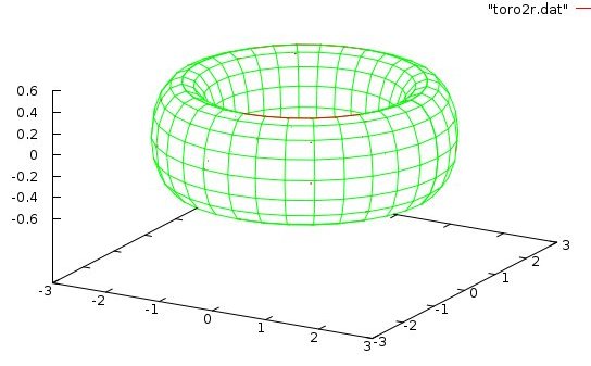
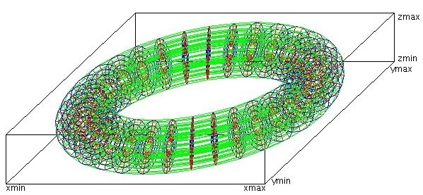 First refinement
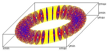 Another view of refinement
Toroid center at 0,0,0 can be translated and rotated
r1, r2, theta, phi mapped to x,y,z
x = (r1+r2*sin(phi))*cos(theta)
y = (r1+r2*sin(phi))*sin(theta)
z = r2 * cos(phi)
0 ≤ theta ≤ 2Pi 0 ≤ phi ≤ 2Pi 0 < r2 < r1
Area = (2*Pi*r1)*(2*Pi*r2) infinitesimal area = dtheta*r1*dphi*r2
Volume = (2*Pi*r1)*(Pi*r2*r2) infinitesimal volume = dtheta*r1*dphi*r2*dr2
Equation (r1-sqrt(x^2+y^2))^2 + z^2 = r2^2
r2, x, y, z mapped to r1, theta, phi (r2 taken as constant)
theta = arctan(y/x)
phi = arccos(z/r2)
r1 = x/cos(theta) - r2*sin(phi) or
r1 = y/sin(theta) - r2*sin(phi) no divide by zero
r1, x, y, z mapped to r2, theta, phi (r1 taken as constant)
theta = arctan(y/x) fix angle by quadrant
x1 = r1*cos(theta)
y1 = r1*sin(theta)
phi = arctan(sqrt((x-x1)^2+(y-y1)^2)/z) fix by quadrant
r2 = sqrt((x-x1)^2+(y-y1)^2+z^2)
PDE for testing: r1 constant, r2 is r, theta is t, phi is p
dU^2(r1,r2,t,p)/dr2^2 + dU^2(r1,r2,t,p)/dt^2 +
dU^2(r1,r2,t,p)/dp^2 = f(r1,r2,t,p)
U(r,t,p):=r*r*(1+sin(t))*(1+cos(p));
2
U(r, t, p) := r (1 + sin(t)) (1 + cos(p))
Urr(r,t,p):=diff(diff(U(r,t.p),r),r);
Urr(r, t, p) := D[1, 1](U)(r, t . p)
Urr(r,t,p):=diff(diff(U(r,t,p),r),r);
Urr(r, t, p) := 2 (1 + sin(t)) (1 + cos(p))
Utt(r,t,p):=diff(diff(U(r,t,p),t),t);
2
Utt(r, t, p) := -r sin(t) (1 + cos(p))
Upp(r,t,p):=diff(diff(U(r,t,p),p),p);
2
Upp(r, t, p) := -r (1 + sin(t)) cos(p)
f(r,t,p):=Urr(r,t,p)+Utt(r,t,p)+Upp(r,t,p);
2
f(r, t, p) := 2 (1 + sin(t)) (1 + cos(p)) - r sin(t) (1 + cos(p))
2
- r (1 + sin(t)) cos(p)
simplify(f(r,t,p));
2 2
2 + 2 cos(p) + 2 sin(t) + 2 sin(t) cos(p) - r sin(t) - 2 r sin(t) cos(p)
2
- r cos(p)
f(r2,t,p) =
2.0*(1.0 + cos(p) + sin(t) + sin(t)*cos(p)) -
r2*r2*(cos(p) + sin(t) + 2.0*sin(t)*cos(p))
Ub(r2,t,p):=r2*r2*(1.0+sin(t))*(1.0+cos(p)); Dirichlet boundary
Another view of refinement
Toroid center at 0,0,0 can be translated and rotated
r1, r2, theta, phi mapped to x,y,z
x = (r1+r2*sin(phi))*cos(theta)
y = (r1+r2*sin(phi))*sin(theta)
z = r2 * cos(phi)
0 ≤ theta ≤ 2Pi 0 ≤ phi ≤ 2Pi 0 < r2 < r1
Area = (2*Pi*r1)*(2*Pi*r2) infinitesimal area = dtheta*r1*dphi*r2
Volume = (2*Pi*r1)*(Pi*r2*r2) infinitesimal volume = dtheta*r1*dphi*r2*dr2
Equation (r1-sqrt(x^2+y^2))^2 + z^2 = r2^2
r2, x, y, z mapped to r1, theta, phi (r2 taken as constant)
theta = arctan(y/x)
phi = arccos(z/r2)
r1 = x/cos(theta) - r2*sin(phi) or
r1 = y/sin(theta) - r2*sin(phi) no divide by zero
r1, x, y, z mapped to r2, theta, phi (r1 taken as constant)
theta = arctan(y/x) fix angle by quadrant
x1 = r1*cos(theta)
y1 = r1*sin(theta)
phi = arctan(sqrt((x-x1)^2+(y-y1)^2)/z) fix by quadrant
r2 = sqrt((x-x1)^2+(y-y1)^2+z^2)
PDE for testing: r1 constant, r2 is r, theta is t, phi is p
dU^2(r1,r2,t,p)/dr2^2 + dU^2(r1,r2,t,p)/dt^2 +
dU^2(r1,r2,t,p)/dp^2 = f(r1,r2,t,p)
U(r,t,p):=r*r*(1+sin(t))*(1+cos(p));
2
U(r, t, p) := r (1 + sin(t)) (1 + cos(p))
Urr(r,t,p):=diff(diff(U(r,t.p),r),r);
Urr(r, t, p) := D[1, 1](U)(r, t . p)
Urr(r,t,p):=diff(diff(U(r,t,p),r),r);
Urr(r, t, p) := 2 (1 + sin(t)) (1 + cos(p))
Utt(r,t,p):=diff(diff(U(r,t,p),t),t);
2
Utt(r, t, p) := -r sin(t) (1 + cos(p))
Upp(r,t,p):=diff(diff(U(r,t,p),p),p);
2
Upp(r, t, p) := -r (1 + sin(t)) cos(p)
f(r,t,p):=Urr(r,t,p)+Utt(r,t,p)+Upp(r,t,p);
2
f(r, t, p) := 2 (1 + sin(t)) (1 + cos(p)) - r sin(t) (1 + cos(p))
2
- r (1 + sin(t)) cos(p)
simplify(f(r,t,p));
2 2
2 + 2 cos(p) + 2 sin(t) + 2 sin(t) cos(p) - r sin(t) - 2 r sin(t) cos(p)
2
- r cos(p)
f(r2,t,p) =
2.0*(1.0 + cos(p) + sin(t) + sin(t)*cos(p)) -
r2*r2*(cos(p) + sin(t) + 2.0*sin(t)*cos(p))
Ub(r2,t,p):=r2*r2*(1.0+sin(t))*(1.0+cos(p)); Dirichlet boundary
Go over WEB pages Lecture 1 through 29, including:
                  3a, 3b, 18a, 24a, 24b, 27a and 28a.
Open book, open notes
Read the instructions.
Follow the instructions, else lose points.
Read the question carefully.
Answer the question that is asked, not the question you want to answer.

Go over Quiz1 and Quiz2. Some of those questions may be reused.
Go over Lecture 9 Review, Lecture 19 Review.

Things you should know:

It is best to find working code to do the numerical computation that
you need, rather than to develop the code yourself.

Thoroughly test any numerical code you are planning to use.

Convert existing, tested, numerical code to the language of your choice.

It is usually better to convert working numerical code to the language
of your choice, rather than creating a multi language interface.
(The exception to this suggestion is LAPACK.)

Modify the interfaces as needed for your application.

Do not put trust in benchmarks that others have run. Run your own benchmarks.

It is possible for operating system code or library code to have an
error that causes incorrect time for a benchmark.

A benchmark must run long enough to avoid error due to the hardware
or software quantization of time. Ten seconds has been found acceptable
on most computers. Less that one second has been found to be bad on
a few computers.

Dead code elimination can cause a benchmark to appear to run very fast.
Using an "if" statement or "print" statement of computed variable
can prevent dead code elimination.

If you are unable to run a benchmark yourself, try to find benchmarks
that resembles what you are interested in.

It is possible to computer derivatives very accurately with high
order equations. A function is available in a few languages to
compute the required coefficients.

Derivatives can be computed for any function that can be evaluated.
By using more function evaluations, better accuracy can be obtained.
Making the step size extremely small may hurt accuracy.

A second derivative can be computed by numerically computing two
successive first derivatives. Yet, accuracy will be better when
using the formulas for second order derivatives.

More function evaluations are required in order to maintain the
same order of accuracy for each higher derivative.

Ordinary differential equations have only one independent variable.

Partial differential equations have more than one independent variable.

The "order" of a differential equation is the highest derivative in
the equation.

The "degree" of a differential equation is the highest power of
any combinations of variables and unknown solution.

The "dimension" of a differential equation is the number of
independent variables.

"initial value" problems have enough information to start
computing the solution from the initial point in every dimension.

"boundary value" problems have the solution, Dirchlet, values
given on the boundary of every dimension. The slope, Neumann,
values may also be provided.

Many specific names are given to differential equations:
"parabolic" "diffusion equation" "hyperbolic" "wave equation"
"elliptic" "Laplace's equation" "biharmonic equation" etc.

Given y=f(x) the first derivatives of  f(x)  may be written as
 y'  f'  f'(x)  df/dx .

For partial derivatives, given  z=f(x,y)  dz/dx may be written as  fx,
dz/dy may be written as fy,  d^3z/dx^2 dy man be written  fxxy .
(and may use partial derivative symbol in place of  d )

The Runge-Kutta method is a common way to compute an iterative solution,
initial value problem, to an ordinary differential equation.

Solving a system of linear equations is a common way to compute a
solution to both ordinary and partial differential equations.
Generally, boundary value problems.

The unknowns in the system of differential equations being used
to solve a differential equations are the values of the unknown
function at specific points. e.g. y(h), y(2h), y(3h), etc.

Given a fourth order ordinary differential equation with only
initial conditions, y'''' = f(x), in order to find a unique
numerical solution, values for  c   must be given for:
  c1 = y(x0)  c2 = y'(x0)  c3 = y''(x0)  c4 = y'''(x0)
and all the values must be at the same x0.

A method that might give reasonable results for the above equation can  be:
    x     = x0
    y     = c1
    yp    = c2   yp is for y'
    ypp   = c3
    yppp  = c4
L:  ypppp = f(x)
    yppp  = yppp + h * ypppp
    ypp   = ypp  + h * yppp
    yp    = yp   + h * ypp
    y     = y    + h * yp       this is the solution at  x0+h
    x     = x    + h            loop to L: for more values.
                                could print or save x,y

Much of Lecture 27 and 28 were from the source code:
pde3.c     A second order partial differential equation with
           boundary values, two independent variables, with equal
           step size, using an iterative method.

pde3_eq.c  same as pde3.c with the iteration replaced by a call
           to simeq and the setup of the matrix in init_matrix.

pde3b.c    A similar second order partial differential equation
           with boundary values, three independent variables and
           each independent variable can have a unique step size
           and a unique number of points to be evaluated.

pde3b_eq.c same as pde3b.c with the iteration replaced by a call
           to simeq and the setup of the matrix in init_matrix.

Notice that these programs were also provided in various other
languages and looked very similar.

The problem was provided in the comments and in the code.

These "solvers" had the solution programmed in so that the method
and the code could be tested. In general the solution is not
known. The solution is computed at some specific points. If the
solution is needed at other points, then interpolation is used.

These "solvers" were based on solving a partial differential
equation that was continuous and continuously differentiable.
There are many specialized solvers for specific partial differential
equations. These lectures just covered two of the many methods

You have learned about modeling and simulation

You have worked with physical world modeling and simulation
by numerical computation. This is a valuable skill in helping
your future employer reach good decisions, as shown in the
diagram from SIAM Review.
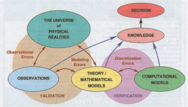
Multiple choice and short answer.
No help from other students, that is cheating!

Read exam carefully! You may think you saw that question
before. Dependent and independent are opposite.
"not" or "no" may have been added or deleted.
"All" and "some" are different.
Do not guess at answer, you can look it up.

I want you to learn to read carefully so you will
do good on your first employment.

You must download quiz3.

last name a-j a, last name k-r b, last name s-z c   ?
cp /afs/umbc.edu/users/s/q/squire/pub/download/q3_455a.doc
cp /afs/umbc.edu/users/s/q/squire/pub/download/q3_455b.doc
cp /afs/umbc.edu/users/s/q/squire/pub/download/q3_455c.doc

Use Microsoft Word  or  libreoffice  to edit.

Then  on linux.gl.umbc.edu
submit cs455 quiz3 q3_455?.doc   or  .docx

Due December 20, 2021
A modified version of fem_50, a Matlab program to use
the Finite Element Method, FEM, to solve a specific
partial differential equation is applied to three very
small test cases with full printout to show the details
of one software implementation.
The differential equation is:
d^2 u(x,y) d^2 u(x,y)
- ---------- - ---------- = f(x,y) or -Uxx(x,y) -Uyy(x,y) = F(x,y)
dx^2 dy^2
For testing, the solution is u(x,y)=1 + 2/11 x^2 + 3/11 y^2
and then f(x,y)= - 10/11
The modified fem_50d.m is also shown below
Case 1 used a triangularization with 6 triangles
7 nodes
6 boundary nodes
1 degree of freedom
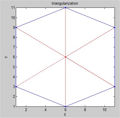 The blue edges and dots are boundary.
The red edges and dots are internal, free.
The one free node is in the center, node number 7.
The full output is A7_fem_50d.out
The solution for the 7 nodes is at the end.
Input files are:
A7_coord.dat
A7_elem3.dat
A7_dirich.dat
The files A7_elem4.dat and A7_neum.dat exists and are empty.
The solution plot is:
The blue edges and dots are boundary.
The red edges and dots are internal, free.
The one free node is in the center, node number 7.
The full output is A7_fem_50d.out
The solution for the 7 nodes is at the end.
Input files are:
A7_coord.dat
A7_elem3.dat
A7_dirich.dat
The files A7_elem4.dat and A7_neum.dat exists and are empty.
The solution plot is:
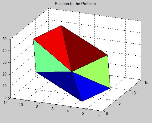 Case 2 used a triangularization with 16 triangles
15 nodes
12 boundary nodes
3 degrees of freedom
Case 2 used a triangularization with 16 triangles
15 nodes
12 boundary nodes
3 degrees of freedom
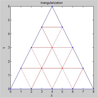 The blue edges and dots are boundary.
The red edges and dots are internal, free.
The three free nodes are in the center, number 13, 14, 15
The full output is A15_fem_50d.out
The solution for the 15 nodes is at the end.
Input files are:
A15_coord.dat
A15_elem3.dat
A15_dirich.dat
The files A15_elem4.dat and A15_neum.dat exists and are empty.
The solution plot is:
The blue edges and dots are boundary.
The red edges and dots are internal, free.
The three free nodes are in the center, number 13, 14, 15
The full output is A15_fem_50d.out
The solution for the 15 nodes is at the end.
Input files are:
A15_coord.dat
A15_elem3.dat
A15_dirich.dat
The files A15_elem4.dat and A15_neum.dat exists and are empty.
The solution plot is:
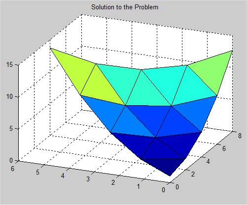 Case 3 used a triangularization with 18 triangles
16 nodes
12 boundary nodes
4 degrees of freedom
Case 3 used a triangularization with 18 triangles
16 nodes
12 boundary nodes
4 degrees of freedom
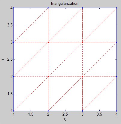 The blue edges and dots are boundary.
The red edges and dots are internal, free.
The four free nodes are in the center, numbered 1, 2, 3, 4
The full output is A16_fem_50d.out
The solution for the 16 nodes is at the end.
Input files are:
A16_coord.dat
A16_elem3.dat
A16_dirich.dat
The files A16_elem4.dat and A16_neum.dat exists and are empty.
The solution plot is:
The blue edges and dots are boundary.
The red edges and dots are internal, free.
The four free nodes are in the center, numbered 1, 2, 3, 4
The full output is A16_fem_50d.out
The solution for the 16 nodes is at the end.
Input files are:
A16_coord.dat
A16_elem3.dat
A16_dirich.dat
The files A16_elem4.dat and A16_neum.dat exists and are empty.
The solution plot is:
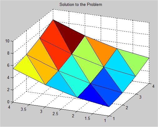 The original fem_50.m all in one file with lots of output added
%% fem_50d applies the finite element method to Laplace's equation.
function fem_50d
% input a prefix, e.g. A7_
% files read A7_coord.dat one x y pair per line, for nodes in order 1, 2, ...
% A7_elem3.dat three node numbers per line, triangles, any order
% function stima3 is applied to these cooddinates
% A7_elem4.dat four node numbers per line, quadralaterals
% function stima4 is applied to these coordinates
% A7_dirich.dat two node numbers per line, dirichlet boundary
% function u_d is applied to these coordinates
% A7_neum.dat two node numbers per line, neumann bounday
% function g is applied to these coordinates
%
% Discussion:
% FEM_50d is a set of MATLAB routines to apply the finite
% element method to solving Laplace's equation in an arbitrary
% region, using about 50 lines of MATLAB code.
%
% FEM_50d is partly a demonstration, to show how little it
% takes to implement the finite element method (at least using
% every possible MATLAB shortcut.) The user supplies datafiles
% that specify the geometry of the region and its arrangement
% into triangular and quadrilateral elements, and the location
% and type of the boundary conditions, which can be any mixture
% of Neumann and dirichlet.
%
% The unknown state variable U(x,y) is assumed to satisfy
% Laplace's equation:
% -Uxx(x,y) - Uyy(x,y) = F(x,y) in Omega
% with dirichlet boundary conditions
% U(x,y) = U_D(x,y) on Gamma_D
% and Neumann boundary conditions on the outward normal derivative:
% Un(x,y) = G(x,y) on Gamma_N
% If Gamma designates the boundary of the region Omega,
% then we presume that
% Gamma = Gamma_D + Gamma_N
% but the user is free to determine which boundary conditions to
% apply. Note, however, that the problem will generally be singular
% unless at least one dirichlet boundary condition is specified.
%
% The code uses piecewise linear basis functions for triangular elements,
% and piecewise isoparametric bilinear basis functions for quadrilateral
% elements.
%
% The user is required to supply a number of data files and MATLAB
% functions that specify the location of nodes, the grouping of nodes
% into elements, the location and value of boundary conditions, and
% the right hand side function in Laplace's equation. Note that the
% fact that the geometry is completely up to the user means that
% just about any two dimensional region can be handled, with arbitrary
% shape, including holes and islands.
%
% Modified:
% 29 March 2004
% 23 February 2008 JSS
% 3 March 2008 JSS
% Reference:
% Jochen Alberty, Carsten Carstensen, Stefan Funken,
% Remarks Around 50 Lines of MATLAB:
% Short Finite Element Implementation,
% Numerical Algorithms,
% Volume 20, pages 117-137, 1999.
%
clear
format compact
prename = input('enter prefix to file names: ', 's')
diary 'fem_50d.out'
disp([prename 'fem_50d.out'])
debug = input('enter debug level:0=none, 1=input and matrices, 2=assembly ')
%
% Read the nodal coordinatesinate data file.
% ordered list of x y pairs, coordinates for nodes
% nodes must be sequentially numbered 1, 2, 3, ...
coordinates = load(strcat(prename,'coord.dat'));
if debug>0
disp([prename 'coord.dat ='])
disp(coordinates)
end % debug
%
% Read the triangular element data file.
% three integer node numbers per line
elements3 = load(strcat(prename,'elem3.dat'));
if debug>0
disp([prename 'elem3.dat ='])
disp(elements3)
end % debug
%
% Read the quadrilateral element data file.
% four integer node numbers per line
elements4 = load(strcat(prename,'elem4.dat'));
if debug>0
disp([prename 'elem4.dat ='])
disp(elements4)
end % debug
%
% Read the dirichlet boundary edge data file.
% two integer node numbers per line, function u_d sets values
% there must be at least one pair
% other boundary edges are set in neumann
dirichlet = load(strcat(prename,'dirich.dat'));
if debug>0
disp([prename 'dirich.dat ='])
disp(dirichlet)
end % debug
%
% Read the Neumann boundary edge data file.
% two integer node numbers per line, function g sets values
neumann = load(strcat(prename,'neum.dat'));
if debug>0
disp([prename 'neum.dat ='])
disp(neumann)
end % debug
A = sparse ( size(coordinates,1), size(coordinates,1) );
b = sparse ( size(coordinates,1), 1 );
%
% Assembly from triangles.
%
for j = 1 : size(elements3,1)
VV = coordinates(elements3(j,:),:);
MM = stima3(coordinates(elements3(j,:),:));
if debug>1
disp(['MM = stima3(VV) at j=' num2str(j) ' nodes(' ...
num2str(elements3(j,1)) ',' num2str(elements3(j,2)) ',' ...
num2str(elements3(j,3)) ')'])
disp('VV=')
disp(VV)
disp('MM=')
disp(MM)
end % debug
A(elements3(j,:),elements3(j,:)) = A(elements3(j,:),elements3(j,:)) + MM;
end
if debug>0
disp('assembly from triangles A=')
disp(A)
end % debug
%
% Assembly from quadralaterals.
%
for j = 1 : size(elements4,1)
VV = coordinates(elements3(j,:),:);
MM = stima4(coordinates(elements4(j,:),:));
if debug>1
disp(['MM = stima3(VV) at j=' num2str(j) ' nodes(' ...
num2str(elements4(j,1)) ',' num2str(elements4(j,2)) ',' ...
num2str(elements4(j,3)) ',' num2str(elements4(j,4)) ')'])
disp('VV=')
disp(VV)
disp('MM=')
disp(MM)
end % debug
A(elements4(j,:),elements4(j,:)) = A(elements4(j,:),elements4(j,:)) + MM;
end
if debug>0
disp('assembly from triangles and rectangles A=')
disp(A)
end % debug
%
% Volume Forces from triangles.
%
for j = 1 : size(elements3,1)
b(elements3(j,:)) = b(elements3(j,:)) ...
+ det( [1,1,1; coordinates(elements3(j,:),:)'] ) * ...
f(sum(coordinates(elements3(j,:),:))/3)/6;
end
if debug>0
disp('forces from triangles b=')
disp(b)
end % debug
%
% Volume Forces from quadralaterals.
%
for j = 1 : size(elements4,1)
b(elements4(j,:)) = b(elements4(j,:)) ...
+ det([1,1,1; coordinates(elements4(j,1:3),:)'] ) * ...
f(sum(coordinates(elements4(j,:),:))/4)/4;
end
if debug>0
disp('forces from triangles and rectangles b=')
disp(b)
end % debug
%
% Neumann conditions.
%
for j = 1 : size(neumann,1)
GG = norm(coordinates(neumann(j,1),:) - coordinates(neumann(j,2),:)) * ...
g(sum(coordinates(neumann(j,:),:))/2)/2;
if debug>2
disp(['Neumann at j=' num2str(j)])
disp(GG)
end % debug
b(neumann(j,:)) = b(neumann(j,:)) + GG
end
if debug>0
disp('using g() add neumann conditions b=')
disp(b)
end % debug
%
% Determine which nodes are associated with dirichlet conditions.
% Assign the corresponding entries of U, and adjust the right hand side.
%
u = sparse ( size(coordinates,1), 1 );
BoundNodes = unique ( dirichlet );
if debug>1
disp('BoundNodes=')
disp(BoundNodes)
end % debug
u(BoundNodes) = u_d ( coordinates(BoundNodes,:) );
if debug>0
disp('using u_d() add dirichlet conditions u=')
disp(u)
end % debug
b = b - A * u;
if debug>0
disp('apply u to b, dirichlet conditions b=')
disp(b)
end % debug
%
% Compute the solution by solving A * u = b
% for the, un bound, remaining unknown values of u.
%
FreeNodes = setdiff ( 1:size(coordinates,1), BoundNodes );
u(FreeNodes) = A(FreeNodes,FreeNodes) \ b(FreeNodes);
if debug>0
disp('solve for A * u = b u=')
disp(u)
end % debug
%
% Graphic representation.
%
show ( elements3, elements4, coordinates, full(u), dirichlet );
%
% check solution
%
for i=1:size(coordinates,1)
disp([num2str(i) ' x= ' num2str(coordinates(i,1)) ' y= ' num2str(coordinates(i,2)) ...
' analytic solution= ' num2str(uana(coordinates(i,1),coordinates(i,2)))])
end
diary off
return % logical end of function fem_50d
%% uana computes boundary values and analytic solution for checking
% Discussion:
% This is generally unknown yet is used here for testing
% Parameters:
% Input, real pair xx,yy are x,y coordinates
% Output, value of solution at x,y
%
function ana = uana(xx, yy)
ana= 1.0+(2.0/11.0)*xx*xx+(3.0/11.0)*yy*yy;
end % uana
%% f evaluates the right hand side of Laplace's equation.
% Discussion:
% This routine must be changed by the user to reflect a particular problem.
% Parameters:
% Input, real U(N,M), contains the M-dimensional coordinates of N points.
% Output, VALUE(N), contains the value of the right hand side of Laplace's
% equation at each of the points.
function valuef = f ( uf )
valuef = ones ( size ( uf, 1 ), 1 );
valuef = valuef.*(-10/11.0);
end % f
%% g evaluates the outward normal values assigned at Neumann boundary conditions.
% Discussion:
% This routine must be changed by the user to reflect a particular problem.
% Parameters:
% Input, real U(N,M), contains the M-dimensional coordinates of N points.
% Output, VALUE(N), contains the value of outward normal at each point
% where a Neumann boundary condition is applied.
function valueg = g ( ug )
valueg = zeros ( size ( ug, 1 ), 1 );
end % g
%% u_d evaluates the dirichlet boundary conditions.
% Discussion:
% The user must supply the appropriate routine for a given problem
% Parameters:
% Input, real U(N,M), contains the M-dimensional coordinates of N points.
% Output, VALUE(N), contains the value of the dirichlet boundary
% condition at each point.
function valued = u_d ( ud )
valued = zeros ( size ( ud, 1 ), 1 );
for kk=1:size(ud,1)
% U(x,y) = 1 + 2/11 x^2 + 3/11 y^2 solution values on boundary
valued(kk)=uana(ud(kk,1),ud(kk,2));
end
end % u_d
%% STIMA3 determines the local stiffness matrix for a triangular element.
% Discussion:
%
% Although this routine is intended for 2D usage, the same formulas
% work for tetrahedral elements in 3D. The spatial dimension intended
% is determined implicitly, from the spatial dimension of the vertices.
% Parameters:
%
% Input, real VERTICES(1:(D+1),1:D), contains the D-dimensional
% coordinates of the vertices.
%
% Output, real M(1:(D+1),1:(D+1)), the local stiffness matrix
% for the element.
function M = stima3 ( vertices )
d = size ( vertices, 2 );
D_eta = [ ones(1,d+1); vertices' ] \ [ zeros(1,d); eye(d) ];
M = det ( [ ones(1,d+1); vertices' ] ) * D_eta * D_eta' / prod ( 1:d );
end % stima3
%% STIMA4 determines the local stiffness matrix for a quadrilateral element.
% Parameters:
% Input, real VERTICES(1:4,1:2), contains the coordinates of the vertices.
% Output, real M(1:4,1:4), the local stiffness matrix for the element.%
function M = stima4 ( vertices )
D_Phi = [ vertices(2,:) - vertices(1,:); vertices(4,:) - vertices(1,:) ]';
B = inv ( D_Phi' * D_Phi );
C1 = [ 2, -2; -2, 2 ] * B(1,1) ...
+ [ 3, 0; 0, -3 ] * B(1,2) ...
+ [ 2, 1; 1, 2 ] * B(2,2);
C2 = [ -1, 1; 1, -1 ] * B(1,1) ...
+ [ -3, 0; 0, 3 ] * B(1,2) ...
+ [ -1, -2; -2, -1 ] * B(2,2);
M = det ( D_Phi ) * [ C1 C2; C2 C1 ] / 6;
end % stima4
%% SHOW displays the solution of the finite element computation.
% Parameters:
% Input, integer elements3(N3,3), the nodes that make up each triangle.
% Input, integer elements4(N4,4), the nodes that make up each quadrilateral.
% Input, real coordinates(N,1:2), the coordinates of each node.
% Input, real U(N), the finite element coefficients which represent the solution.
% There is one coefficient associated with each node.
function show ( elements3, elements4, coordinates, us, dirichlet )
figure(1)
hold off
%
% Display the information associated with triangular elements.
trisurf ( elements3, coordinates(:,1), coordinates(:,2), us' );
%
% Retain the previous image, and overlay the information associated
% with quadrilateral elements.
hold on
trisurf ( elements4, coordinates(:,1), coordinates(:,2), us' );
%
% Define the initial viewing angle.
%
view ( -67.5, 30 );
title ( 'Solution to the Problem' )
hold off
figure(2)
for kk=1:size(elements3,1)
plot([coordinates(elements3(kk,1),1) ...
coordinates(elements3(kk,2),1) ...
coordinates(elements3(kk,3),1) ...
coordinates(elements3(kk,1),1)], ...
[coordinates(elements3(kk,1),2) ...
coordinates(elements3(kk,2),2) ...
coordinates(elements3(kk,3),2) ...
coordinates(elements3(kk,1),2)],':r')
hold on
end
for kk=1:size(dirichlet,1)
plot([coordinates(dirichlet(kk,1),1) ...
coordinates(dirichlet(kk,2),1)], ...
[coordinates(dirichlet(kk,1),2) ...
coordinates(dirichlet(kk,2),2)],'-b')
hold on
end
title('triangularization')
xlabel('X')
ylabel('Y')
axis tight
axis square
grid off
hold on
xb=coordinates(BoundNodes,1);
yb=coordinates(BoundNodes,2);
plot(xb,yb,'.b')
hold on
xb=coordinates(FreeNodes,1);
yb=coordinates(FreeNodes,2);
plot(xb,yb,'.r')
hold off
end % show
end % fem_50d
The original fem_50.m all in one file with lots of output added
%% fem_50d applies the finite element method to Laplace's equation.
function fem_50d
% input a prefix, e.g. A7_
% files read A7_coord.dat one x y pair per line, for nodes in order 1, 2, ...
% A7_elem3.dat three node numbers per line, triangles, any order
% function stima3 is applied to these cooddinates
% A7_elem4.dat four node numbers per line, quadralaterals
% function stima4 is applied to these coordinates
% A7_dirich.dat two node numbers per line, dirichlet boundary
% function u_d is applied to these coordinates
% A7_neum.dat two node numbers per line, neumann bounday
% function g is applied to these coordinates
%
% Discussion:
% FEM_50d is a set of MATLAB routines to apply the finite
% element method to solving Laplace's equation in an arbitrary
% region, using about 50 lines of MATLAB code.
%
% FEM_50d is partly a demonstration, to show how little it
% takes to implement the finite element method (at least using
% every possible MATLAB shortcut.) The user supplies datafiles
% that specify the geometry of the region and its arrangement
% into triangular and quadrilateral elements, and the location
% and type of the boundary conditions, which can be any mixture
% of Neumann and dirichlet.
%
% The unknown state variable U(x,y) is assumed to satisfy
% Laplace's equation:
% -Uxx(x,y) - Uyy(x,y) = F(x,y) in Omega
% with dirichlet boundary conditions
% U(x,y) = U_D(x,y) on Gamma_D
% and Neumann boundary conditions on the outward normal derivative:
% Un(x,y) = G(x,y) on Gamma_N
% If Gamma designates the boundary of the region Omega,
% then we presume that
% Gamma = Gamma_D + Gamma_N
% but the user is free to determine which boundary conditions to
% apply. Note, however, that the problem will generally be singular
% unless at least one dirichlet boundary condition is specified.
%
% The code uses piecewise linear basis functions for triangular elements,
% and piecewise isoparametric bilinear basis functions for quadrilateral
% elements.
%
% The user is required to supply a number of data files and MATLAB
% functions that specify the location of nodes, the grouping of nodes
% into elements, the location and value of boundary conditions, and
% the right hand side function in Laplace's equation. Note that the
% fact that the geometry is completely up to the user means that
% just about any two dimensional region can be handled, with arbitrary
% shape, including holes and islands.
%
% Modified:
% 29 March 2004
% 23 February 2008 JSS
% 3 March 2008 JSS
% Reference:
% Jochen Alberty, Carsten Carstensen, Stefan Funken,
% Remarks Around 50 Lines of MATLAB:
% Short Finite Element Implementation,
% Numerical Algorithms,
% Volume 20, pages 117-137, 1999.
%
clear
format compact
prename = input('enter prefix to file names: ', 's')
diary 'fem_50d.out'
disp([prename 'fem_50d.out'])
debug = input('enter debug level:0=none, 1=input and matrices, 2=assembly ')
%
% Read the nodal coordinatesinate data file.
% ordered list of x y pairs, coordinates for nodes
% nodes must be sequentially numbered 1, 2, 3, ...
coordinates = load(strcat(prename,'coord.dat'));
if debug>0
disp([prename 'coord.dat ='])
disp(coordinates)
end % debug
%
% Read the triangular element data file.
% three integer node numbers per line
elements3 = load(strcat(prename,'elem3.dat'));
if debug>0
disp([prename 'elem3.dat ='])
disp(elements3)
end % debug
%
% Read the quadrilateral element data file.
% four integer node numbers per line
elements4 = load(strcat(prename,'elem4.dat'));
if debug>0
disp([prename 'elem4.dat ='])
disp(elements4)
end % debug
%
% Read the dirichlet boundary edge data file.
% two integer node numbers per line, function u_d sets values
% there must be at least one pair
% other boundary edges are set in neumann
dirichlet = load(strcat(prename,'dirich.dat'));
if debug>0
disp([prename 'dirich.dat ='])
disp(dirichlet)
end % debug
%
% Read the Neumann boundary edge data file.
% two integer node numbers per line, function g sets values
neumann = load(strcat(prename,'neum.dat'));
if debug>0
disp([prename 'neum.dat ='])
disp(neumann)
end % debug
A = sparse ( size(coordinates,1), size(coordinates,1) );
b = sparse ( size(coordinates,1), 1 );
%
% Assembly from triangles.
%
for j = 1 : size(elements3,1)
VV = coordinates(elements3(j,:),:);
MM = stima3(coordinates(elements3(j,:),:));
if debug>1
disp(['MM = stima3(VV) at j=' num2str(j) ' nodes(' ...
num2str(elements3(j,1)) ',' num2str(elements3(j,2)) ',' ...
num2str(elements3(j,3)) ')'])
disp('VV=')
disp(VV)
disp('MM=')
disp(MM)
end % debug
A(elements3(j,:),elements3(j,:)) = A(elements3(j,:),elements3(j,:)) + MM;
end
if debug>0
disp('assembly from triangles A=')
disp(A)
end % debug
%
% Assembly from quadralaterals.
%
for j = 1 : size(elements4,1)
VV = coordinates(elements3(j,:),:);
MM = stima4(coordinates(elements4(j,:),:));
if debug>1
disp(['MM = stima3(VV) at j=' num2str(j) ' nodes(' ...
num2str(elements4(j,1)) ',' num2str(elements4(j,2)) ',' ...
num2str(elements4(j,3)) ',' num2str(elements4(j,4)) ')'])
disp('VV=')
disp(VV)
disp('MM=')
disp(MM)
end % debug
A(elements4(j,:),elements4(j,:)) = A(elements4(j,:),elements4(j,:)) + MM;
end
if debug>0
disp('assembly from triangles and rectangles A=')
disp(A)
end % debug
%
% Volume Forces from triangles.
%
for j = 1 : size(elements3,1)
b(elements3(j,:)) = b(elements3(j,:)) ...
+ det( [1,1,1; coordinates(elements3(j,:),:)'] ) * ...
f(sum(coordinates(elements3(j,:),:))/3)/6;
end
if debug>0
disp('forces from triangles b=')
disp(b)
end % debug
%
% Volume Forces from quadralaterals.
%
for j = 1 : size(elements4,1)
b(elements4(j,:)) = b(elements4(j,:)) ...
+ det([1,1,1; coordinates(elements4(j,1:3),:)'] ) * ...
f(sum(coordinates(elements4(j,:),:))/4)/4;
end
if debug>0
disp('forces from triangles and rectangles b=')
disp(b)
end % debug
%
% Neumann conditions.
%
for j = 1 : size(neumann,1)
GG = norm(coordinates(neumann(j,1),:) - coordinates(neumann(j,2),:)) * ...
g(sum(coordinates(neumann(j,:),:))/2)/2;
if debug>2
disp(['Neumann at j=' num2str(j)])
disp(GG)
end % debug
b(neumann(j,:)) = b(neumann(j,:)) + GG
end
if debug>0
disp('using g() add neumann conditions b=')
disp(b)
end % debug
%
% Determine which nodes are associated with dirichlet conditions.
% Assign the corresponding entries of U, and adjust the right hand side.
%
u = sparse ( size(coordinates,1), 1 );
BoundNodes = unique ( dirichlet );
if debug>1
disp('BoundNodes=')
disp(BoundNodes)
end % debug
u(BoundNodes) = u_d ( coordinates(BoundNodes,:) );
if debug>0
disp('using u_d() add dirichlet conditions u=')
disp(u)
end % debug
b = b - A * u;
if debug>0
disp('apply u to b, dirichlet conditions b=')
disp(b)
end % debug
%
% Compute the solution by solving A * u = b
% for the, un bound, remaining unknown values of u.
%
FreeNodes = setdiff ( 1:size(coordinates,1), BoundNodes );
u(FreeNodes) = A(FreeNodes,FreeNodes) \ b(FreeNodes);
if debug>0
disp('solve for A * u = b u=')
disp(u)
end % debug
%
% Graphic representation.
%
show ( elements3, elements4, coordinates, full(u), dirichlet );
%
% check solution
%
for i=1:size(coordinates,1)
disp([num2str(i) ' x= ' num2str(coordinates(i,1)) ' y= ' num2str(coordinates(i,2)) ...
' analytic solution= ' num2str(uana(coordinates(i,1),coordinates(i,2)))])
end
diary off
return % logical end of function fem_50d
%% uana computes boundary values and analytic solution for checking
% Discussion:
% This is generally unknown yet is used here for testing
% Parameters:
% Input, real pair xx,yy are x,y coordinates
% Output, value of solution at x,y
%
function ana = uana(xx, yy)
ana= 1.0+(2.0/11.0)*xx*xx+(3.0/11.0)*yy*yy;
end % uana
%% f evaluates the right hand side of Laplace's equation.
% Discussion:
% This routine must be changed by the user to reflect a particular problem.
% Parameters:
% Input, real U(N,M), contains the M-dimensional coordinates of N points.
% Output, VALUE(N), contains the value of the right hand side of Laplace's
% equation at each of the points.
function valuef = f ( uf )
valuef = ones ( size ( uf, 1 ), 1 );
valuef = valuef.*(-10/11.0);
end % f
%% g evaluates the outward normal values assigned at Neumann boundary conditions.
% Discussion:
% This routine must be changed by the user to reflect a particular problem.
% Parameters:
% Input, real U(N,M), contains the M-dimensional coordinates of N points.
% Output, VALUE(N), contains the value of outward normal at each point
% where a Neumann boundary condition is applied.
function valueg = g ( ug )
valueg = zeros ( size ( ug, 1 ), 1 );
end % g
%% u_d evaluates the dirichlet boundary conditions.
% Discussion:
% The user must supply the appropriate routine for a given problem
% Parameters:
% Input, real U(N,M), contains the M-dimensional coordinates of N points.
% Output, VALUE(N), contains the value of the dirichlet boundary
% condition at each point.
function valued = u_d ( ud )
valued = zeros ( size ( ud, 1 ), 1 );
for kk=1:size(ud,1)
% U(x,y) = 1 + 2/11 x^2 + 3/11 y^2 solution values on boundary
valued(kk)=uana(ud(kk,1),ud(kk,2));
end
end % u_d
%% STIMA3 determines the local stiffness matrix for a triangular element.
% Discussion:
%
% Although this routine is intended for 2D usage, the same formulas
% work for tetrahedral elements in 3D. The spatial dimension intended
% is determined implicitly, from the spatial dimension of the vertices.
% Parameters:
%
% Input, real VERTICES(1:(D+1),1:D), contains the D-dimensional
% coordinates of the vertices.
%
% Output, real M(1:(D+1),1:(D+1)), the local stiffness matrix
% for the element.
function M = stima3 ( vertices )
d = size ( vertices, 2 );
D_eta = [ ones(1,d+1); vertices' ] \ [ zeros(1,d); eye(d) ];
M = det ( [ ones(1,d+1); vertices' ] ) * D_eta * D_eta' / prod ( 1:d );
end % stima3
%% STIMA4 determines the local stiffness matrix for a quadrilateral element.
% Parameters:
% Input, real VERTICES(1:4,1:2), contains the coordinates of the vertices.
% Output, real M(1:4,1:4), the local stiffness matrix for the element.%
function M = stima4 ( vertices )
D_Phi = [ vertices(2,:) - vertices(1,:); vertices(4,:) - vertices(1,:) ]';
B = inv ( D_Phi' * D_Phi );
C1 = [ 2, -2; -2, 2 ] * B(1,1) ...
+ [ 3, 0; 0, -3 ] * B(1,2) ...
+ [ 2, 1; 1, 2 ] * B(2,2);
C2 = [ -1, 1; 1, -1 ] * B(1,1) ...
+ [ -3, 0; 0, 3 ] * B(1,2) ...
+ [ -1, -2; -2, -1 ] * B(2,2);
M = det ( D_Phi ) * [ C1 C2; C2 C1 ] / 6;
end % stima4
%% SHOW displays the solution of the finite element computation.
% Parameters:
% Input, integer elements3(N3,3), the nodes that make up each triangle.
% Input, integer elements4(N4,4), the nodes that make up each quadrilateral.
% Input, real coordinates(N,1:2), the coordinates of each node.
% Input, real U(N), the finite element coefficients which represent the solution.
% There is one coefficient associated with each node.
function show ( elements3, elements4, coordinates, us, dirichlet )
figure(1)
hold off
%
% Display the information associated with triangular elements.
trisurf ( elements3, coordinates(:,1), coordinates(:,2), us' );
%
% Retain the previous image, and overlay the information associated
% with quadrilateral elements.
hold on
trisurf ( elements4, coordinates(:,1), coordinates(:,2), us' );
%
% Define the initial viewing angle.
%
view ( -67.5, 30 );
title ( 'Solution to the Problem' )
hold off
figure(2)
for kk=1:size(elements3,1)
plot([coordinates(elements3(kk,1),1) ...
coordinates(elements3(kk,2),1) ...
coordinates(elements3(kk,3),1) ...
coordinates(elements3(kk,1),1)], ...
[coordinates(elements3(kk,1),2) ...
coordinates(elements3(kk,2),2) ...
coordinates(elements3(kk,3),2) ...
coordinates(elements3(kk,1),2)],':r')
hold on
end
for kk=1:size(dirichlet,1)
plot([coordinates(dirichlet(kk,1),1) ...
coordinates(dirichlet(kk,2),1)], ...
[coordinates(dirichlet(kk,1),2) ...
coordinates(dirichlet(kk,2),2)],'-b')
hold on
end
title('triangularization')
xlabel('X')
ylabel('Y')
axis tight
axis square
grid off
hold on
xb=coordinates(BoundNodes,1);
yb=coordinates(BoundNodes,2);
plot(xb,yb,'.b')
hold on
xb=coordinates(FreeNodes,1);
yb=coordinates(FreeNodes,2);
plot(xb,yb,'.r')
hold off
end % show
end % fem_50d
The message here:
Thoroughly test any software you write or are about to use.
Use tools to generate test when possible.
Generate a test case for a second order PDE with two independent variables.
Make the PDE general by having it be elliptic in some regions,
hyperbolic in some regions and passing through parabolic.
Note: This is for the set of solutions that are continuous and
continuously differentiable. There are many special solutions and
corresponding special solvers that should be used for special cases.
This lecture is about a general case and a general solver.
The solution will be u(x,y).
The notation for derivatives will be
uxx(x,y) second derivative of u(x,y) with respect to x
uxy(x,y) derivative of u(x,y) with respect to x and with respect to y
uyy(x,y) second derivative of u(x,y) with respect to
ux(x,y) derivative of u(x,y) with respect to x
uy(x,y) derivative of u(x,y) with respect to y
We will create functions a1(x,y), b1(x,y), c1(x,y), d1(x,y), e1(x,y) and
f1(x,y).
The PDE we intend to solve, compactly, is:
a1 uxx + b1 uxy + c1 uyy + d1 ux + e1 uy + f1 u = c
The PDE written for computer processing is:
a1(x,y)*uxx(x,y) + b1(x,y)*uxy(x,y) + c1(x,y)*uyy(x,y) +
d1(x,y)*ux(x,y) + e1(x,y)*uy(x,y) + f1(x,y)*u(x,y) = c(x,y)
Yes, we could use algebra to reorganize the PDE, yet we will not.
We choose the functions a1, b1 and c1 such that b1^2 -a1 * c1 is
elliptic, hyperbolic and parabolic in various regions.
a1(x,y) = exp(x/2)*exp(y)/2
b1(x,y) = 0.7/(x*x*y*y + 0.5)
c1(x,y) = (4 - exp(x) - exp(y/2))*2
then we plot b1^2 - a1 * c1 over the x-y plane.
abc.m MatLab to plot a1, b1, c1 and b1^2-a1*c1
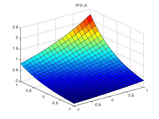
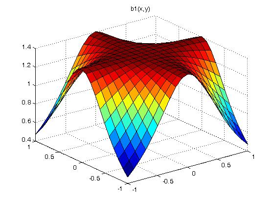
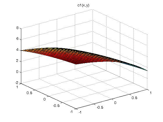
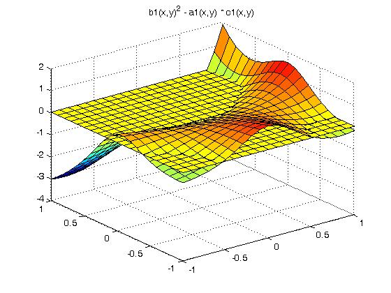 Below the yellow plane is elliptic, above the yellow plane is
hyperbolic and on the yellow plane is parabolic. This has little
to do with the numerical solution of our PDE. For some classic
PDE's only in one region, there are specialized solutions.
Equations of mixed type:
If a PDE has coefficients which are not constant, as shown above,
it is possible that it will not belong to any of the three categories.
A simple but important example is the Euler-Tricomi equation
uxx = xuyy
which is called elliptic-hyperbolic because it is elliptic in the region
x < 0, hyperbolic in the region x > 0, and degenerate parabolic
on the line x = 0.
The other functions for this test case were chosen as:
d1(x,y) = x^2 y
e1(x,y) = x y^2
f1(x,y) = 3x + 2y
Now we have to pick our solution function u(x,y).
Since we will be taking second derivatives, we need at least a
third order solution in order to be interesting.
Out of the air, I chose:
u(x,y) = x^3 + 2y^3 + 3x^2 y + 4xy^2 + 5xy + 6x + 7y + 8
We do not want the solution symmetric in x and y.
We want a smattering of terms for testing.
I use 1, 2, 3, 4, ... to be sure each term tested.
Now we have to compute the forcing function c(x,y)
Doing the computation by hand is too error prone.
I use Maple.
Maple computation of c(x,y) Look at this!
Maple work sheet
Maple output
c(x,y) = 0.5*exp(x/2.0)*exp(y)*(6.0*x+6.0*y) +
0.7*(6.0*x + 8.0*y + 5.0)/(x*x*y*y+0.5) +
(8.0 - 2.0*exp(x) - 2.0*exp(y/2.0))*(12.0*y + 8.0*x) +
(x*x+y)*(3.0*x*x + 6.0*x*y + 4.0*y*y + 5.0*y + 6.0) +
x*y*y*(6.0*y*y + 3.0*x*x + 8.0*x*y + 5.0*x +7.0) +
(3.0*x + 2.0*y)*(x^3 + 2y^3 + 3x^2 y + 4xy^2 + 5xy + 6x + 7y + 8)
We have to code the function c(x,y) for our solver.
We have to code the function u(x,y) for our solver to compute
boundary values and we will use the function to check our solver.
The solution will be u(x,y) and the solver must be able to evaluate
this function on the boundary. The region will be
xmin <= x <= xmax
ymin <= y <= ymax
We will solve for nx points in the x dimension, ny points in y dimension with
hx=(xmax-xmin)/(nx-1) step size in x
hy=(ymax-ymin)/(ny-1) step size in y
We will compute the approximate solution at u(i,j) for the point
u(xmin+i*hx,ymin+j*hy). With subscripts running i=0..nx-1 and j=0..ny-1.
Known boundary values are at i=0, i=nx-1, j=0, and j=ny-1.
These subscripts are for "C" and Java, add one for Ada, Fortran and
MatLab subscripts.
The actual numeric values can be set at the last minute, yet we will
use xmin = ymin = -1.0 xmax = ymax = 1.0 nx = 7 ny = 7
Now, we have to generate the matrix that represents the system of
linear simultaneous equations for the unknown values of u(x,y)
at xmin+i*hx for i=1..nx-2 ymin+j*hy for j=1..ny-2
I am using solution points 1, 2, ... , nx-2 by
1, 2, ... , ny-2 stored in a matrix starting at ut[0][0] for coding in "C".
The solution points will be the same as used in pde3:
The PDE will be made discrete by using unknown values in difference
equations as given in nderiv.out or
computed by deriv.c, deriv.adb, deriv.java, deriv.py, deriv.scala, etc.
For this test case, I choose to use five point derivatives for
both first and second order. Note that the uxy term has the
first derivative with respect to x at five y values then
the first derivative of these values with respect to y.
Taking a term at a time from the PDE and writing the discrete version:
a1(x,y)*uxx(x,y) + b1(x,y)*uxy(x,y) + c1(x,y)*uyy(x,y) +
d1(x,y)*ux(x,y) + e1(x,y)*uy(x,y) + f1(x,y)*u(x,y) = c(x,y)
At (x,y) the discrete approximation of a1(x,y)*uxx(x,y) =
a1(x,y) * (1/(12*hx*hx)) *
(-1*u(x-2hx,y) +16*u(x-hx,y) -30*u(x,y) +16*u(x+hx,y) -1*u(x+2hx,y))
yet, we want to solve for u(i,j) in a matrix,
thus using x=xmin+i*hx and y=ymin+j*hy rewrite the above approximation as
a1(xmin+i*hx,ymin+j*hy) * (1/(12*hx*hx)) *
(-1*u(i-2,j) +16*u(i-1,j) -30*u(i,j) +16*u(i+1,j) -1*u(i+2,j))
At (x,y) c1(x,y)*uyy(x,y) = the discrete approximation
c1(x,y) * (1/(12*hy*hy)) *
(-1*u(x,y-2hy) +16*u(x,y-hy) -30*u(x,y) +16*u(x,y+hy) -1*u(x,y+2hy))
again, we want to solve for u(i,j) in a matrix,
thus using x=xmin+i*hx and y=ymin+j*hy rewrite the above approximation as
c1(xmin+i*hx,ymin+j*hy) * (1/(12*hy*hy)) *
(-1*u(i,j-2) +16*u(i,j-1) -30*u(i,j) +16*u(i,j+1) -1*u(i,j+2))
What happened to b1(x,y)*uxy(x,y) ?
Well that one is more difficult, thus we now use the combination of
the first derivative with respect to x, then the first derivative
with respect to y, 25 terms.
Writing all the terms using i and j
b1(xmin+i*hx,ymin+j*hy) * (1/(144*hx*hy)) *
( 1*u(i-2,j-2) -8*u(i-1,j-2) +0*u(i,j-2) +8*u(i+1,j-2) -1*u(i+2,j-2)
-8*u(i-2,j-1) +64*u(i-1,j-1) +0*u(i,j-1) -64*u(i+1,j-1) +8*u(i+2,j-1)
+0*u(i-2,j ) +0*u(i-1,j ) +0*u(i,j ) +0*u(i+1,j ) +0*u(i+2,j )
+8*u(i-2,j+1) -64*u(i-1,j+1) +0*u(i,j+1) +64*u(i+1,j+1) -8*u(i+2,j+1)
-1*u(i-2,j+2) +8*u(i-1,j+2) +0*u(i,j+2) -8*u(i+1,j+2) +1*u(i+2,j+2))
Just writing the remaining terms using i and j
using the discrete coefficients.
d1(xmin+i*hx,ymin+j*hy) * (1/(12*hx) *
(1*u(i-2,j) -8*u(i-1,j) +0*u(i,j) +8*u(i+1,j) -1*u(i+2,j))
e1(xmin+i*hx,ymin+j*hy) * (1/(12*hy) *
(1*u(i,j-2) -8*u(i,j-1) +0*u(i,j) +8*u(i,j+1) -1*u(i,j+2))
The u(x,y) term is just
f1(xmin+i*hx,ymin+j*hy)*u(i,j)
The right hand side of every approximation above is just
c(xmin+i*hx,ymin+j*hy)
If any of the u(i+a,j+b) are boundary elements, we plug in the
numeric value of the boundary element, multiply by the
coefficient, and subtract the product from the right hand side.
Now we have many equations for u(i,j) using values for i and j,
and we must compute the coefficients for the set of equations
for i=2..nx-3 j=2..ny-3 the central case.
Remember, u(i=0,j), u(i=nx-1,j), u(i,j=0) and u(i,j=ny-1) are
known boundary values.
What about u(1,j), u(nx-2,j) for j=1..ny-2 and
u(i,1), u(i,ny-2) for i=2..nx-3 (do not use u(1,1) twice !!!)
(do not use u(nx-2,ny-2) twice)
Fortunately, the coefficients for the discrete derivatives can be
computed by deriv.c, deriv.adb, etc.
At (1,j) the discrete approximation of
a1(xmin+1*hx,ymin*j*hy)*uxx(xmin+1*hx,ymin+j*hy) =
a1(xmin+1*hx,ymin+j*hy) * (1/(12*hx*hx)) *
(-3*u(i-1,j) -10*u(i,j) +18*u(i+1,j) -6*u(i+2,j) +1*u(i+3,j))
We could not use i-2 because it is outside our region, thus
note "deriv" is called with 'point' set to 1.
At (nx-2,j) the discrete approximation of
a1(xmin+(nx-2)*hx,ymin*j*hy)*uxx(xmin+(nx-2)*hx,ymin+j*hy) =
a1(xmin+(nx-2)*hx,ymin+j*hy) * (1/(12*hx*hx)) *
(-1*u(i-3,j) +6*u(i-2,j) -18*u(i-1,j) +10*u(i,j) +3*u(i+1,j))
We could not use i+2 or (nx-2)+2 because it is outside our region, thus
note "deriv" is called with 'point' set to 3.
There is nothing special about uxx(i,1) or uxx(nx-2,1) use the general case.
At (i,1) the discrete approximation of c1(x,y)*uyy(x,y) =
c1(xmin+i*hx,ymin+1*hy) * (1/(12*hy*hy)) *
(-3*u(i,j-1) -10*u(i,j) +18*u(i,j+1) -6*u(i,j+2) +1*u(i,j+3))
We could not use j-2 because it is outside our region, thus
note "deriv" is called with 'point' set to 1.
At (i,nx-2) the discrete approximation of c1(x,y)*uyy(x,y) =
c1(xmin+i*hx,ymin+(nx-2)*hy) * (1/(12*hy*hy)) *
(-1*u(i,j-3) +6*u(i,j-2) -18*u(i,j-1) +10*u(i,j) +3*u(i,j+1))
We could not use j+2 or (ny-2)+2 because it is outside our region, thus
note "deriv" is called with 'point' set to 3.
There is nothing special about uyy(1,j) or uxx(nx-2,j) use the general case.
Oh, and yes, ux(x,y) uy(x,y) uxy(x,y) also have to be shifted for the
"just inside the boundary case." Think of how much easier it is using five
points rather than sever points. With seven points the two rows and
columns inside the boundary are special cases.
Now we have enough equations to exactly compute the approximate solution.
We build a system of linear equations of the form:
| ut00 ut01 ut02 ut03 | | u(1,1) | | k0 |
| ut10 ut11 ut12 ut13 | * | u(1,2) | = | k1 |
| ut20 ut21 ut22 ut23 | | u(2,1) | | k2 |
| ut30 ut31 ut32 ut33 | | u(2,2) | | k3 |
We know the values at the boundary u(0,0), u(0,1), u(0,2), u(0,3)
u(1,0), u(1,3)
u(2,0), u(2,3)
u(3,0), u(3,1), u(3,2), u(3,3)
For this specific system of equations, nx=4, ny=4 and there are four
internal, non boundary, values to be found. The number of equations
will always be (nx-2)*(ny-2).
The value found for u(1,1) from solving the system of linear equations
is the desired solution at u(xmin+1*hx,ymin+1*hy). u(2,2) is the value of
u(xmin+2*hx,ymin+2*hy). Additional values, not on hx or hy steps,
of u(x,y) may be found by two dimensional interpolation.
The matrix "ut", used in the source code pde_abc_eq.c
is cleared to zero. Then each equation is used and the
coefficient of u(i,j) is added the appropriate ut entry.
There will be (nx-2)*(ny-2) equations that must be used.
The i and j for these equations are for i=1..nx-2 for j=1..ny-2.
The PDE approximation above must be used for these i,j pairs.
Note that u(i,j), u(i-2,j) etc are variables and it is the
coefficients of these variables that get added into the "ut" matrix.
The first equation will add to entries in the first row of the matrix.
The second equation will add to entries in the second row of the matrix.
The boundary values are not stored in the ut matrix and using algebra,
a boundary value coefficient is multiplied by the boundary value and
subtracted from the constant term. This can cause many special cases
in the solver.
In general many entries in a row will not be changed from zero.
The final matrix will be in the class of a band matrix.
Now the gruesome work of evaluating the u(i,j) coefficients.
We cheat here. Now assume nx>4 and ny>5 and thus
i=2, j=3 is a general center case. From above, we have
a1(x,y)*uxx(x,y) + b1(x,y)*uxy(x,y) + c1(x,y)*uyy(x,y) +
d1(x,y)*ux(x,y) + e1(x,y)*uy(x,y) + f1(x,y)*u(x,y) = c(x,y)
converted to a discrete approximation for the central elements is
a1(xmin+i*hx,ymin+j*hy) * (1/(12*hx*hx)) *
(-1*u(i-2,j) +16*u(i-1,j) -30*u(i,j) +16*u(i+1,j) -1*u(i+2,j)) +
b1(xmin+i*hx,y+j*hy) * (1/(144*hx*hy)) *
( 1*u(i-2,j-2) -8*u(i-1,j-2) +0*u(i,j-2) +8*u(i+1,j-2) -1*u(i+2,j-2)
-8*u(i-2,j-1) +64*u(i-1,j-1) +0*u(i,j-1) -64*u(i+1,j-1) +8*u(i+2,j-1)
+0*u(i-2,j ) +0*u(i-1,j ) +0*u(i,j ) +0*u(i+1,j ) +0*u(i+2,j )
+8*u(i-2,j+1) -64*u(i-1,j+1) +0*u(i,j+1) +64*u(i+1,j+1) -8*u(i+2,j+1)
-1*u(i-2,j+2) +8*u(i-1,j+2) +0*u(i,j+2) -8*u(i+1,j+2) +1*u(i+2,j+2)) +
c1(xmin+i*hx,ymin+j*hy) * (1/(12*hy*hy)) *
(-1*u(i,j-2) +16*u(i,j-1) -30*u(i,j) +16*u(i,j+1) -1*u(i,j+2)) +
d1(xmin+i*hx,ymin+j*hy) * (1/(12*hx) *
(1*u(i-2,j) -8*u(i-1,j) +0*u(i,j) +8*u(i+1,j) -1*u(i+2,j)) +
e1(xmin+i*hx,ymin+j*hy) * (1/(12*hy) *
(1*u(i,j-2) -8*u(i,j-1) +0*u(i,j) +8*u(i,j+1) -1*u(i,j+2)) +
f1(xmin+i*hx,ymin+j*hy)*u(i,j) =
c(xmin+i*hx,ymin+j*hy)
Collecting terms for u(i,j) we compute the coefficient ct
a1(xmin+i*hx,ymin+j*hy) * (1/(12*hx*hx)) *(-30) +
b1(xmin+i*hx,ymin+j*hy) * (1/(144*hx*hy)) *(0) +
c1(xmin+i*hx,ymin+j*hy) * (1/(12*hy*hy)) *(-30) +
d1(xmin+i*hx,ymin+j*hy) * (1/(12*hx) *(0) +
e1(xmin+i*hx,ymin+j*hy) * (1/(12*hy) *(0)
and the right hand side is c(xmin+i*hx,ymin+j*hy)
A bit of bizarre subscripting, assuming we are at i=2, j=3 this
is equation number ii=(i-1)+(nx-2)*(j-1), right?
Check i=1,j=1 is equation 0 if i or j equal zero, we have a boundary
i=2,j=1 is equation 1
...
i=nx-2,j=1 is equation nx-3
i=1,j=2 is equation nx-2
i=2,j=2 is equation nx-1
...
i=2,j=3 is equation (2-1)+(nx-2)*(3-1) the row in the ut matrix.
cs, the subscript for the right hand side is cs=(nx-2)*(ny-2) stored in ut.
Thus we add ct to ut(ii,ii). The second subscript is where u(i,j) is.
Well, to tell the truth, we add each component of the sum in a loop,
directly into ut(ii,ii). If we had ct we would just store it in ut(ii,ii).
ut(ii,cs) is set to c(xmin+i*hx,ymin+j*hy) - f1(xmin+i*hx,ymin+j*hy)
We must, of course, compute all the coefficients, e.g. u(i-1,j), ctm1
a1(xmin+i*hx,ymin+j*hy) * (1/(12*hx*hx)) *(16) +
b1(xmin+i*hx,ymin+j*hy) * (1/(144*hx*hy)) *(0) +
c1(xmin+i*hx,ymin+j*hy) * (1/(12*hy*hy)) *(0) + does not exists
d1(xmin+i*hx,ymin+j*hy) * (1/(12*hx) *(-8) +
e1(xmin+i*hx,ymin+j*hy) * (1/(12*hy) *(0) does not exists
ij=(((i-1)-1)+(nx-2)*(j-1) where u(i-1,j) is in the solution vector.
ut(ii,ij) = ctm1
We must, of course, compute all the coefficients, e.g. u(i-2,j), ctmm1
a1(xmin+i*hx,ymin+j*hy) * (1/(12*hx*hy)) *(-1) +
b1(xmin+i*hx,ymin+j*hy) * (1/(144*hx*hy)) *(0) +
c1(xmin+i*hx,ymin+j*hy) * (1/(12*hy*hy)) *(0) + does not exists
d1(xmin+i*hx,ymin+j*hy) * (1/(12*hx) *(1) +
e1(xmin+i*hx,ymin+j*hy) * (1/(12*hy) *(0) does not exists
ij=(((i-2)-1)+(nx-2)*(j-1) where u(i-2,j) is in the solution vector.
ut(ii,ij) = ctmm1 Wrong if i is 2! u(0,j) is a boundary value, thus
ut(ii,cs) = ut(ii,cs) - ctmm1 * u(0,j)
And, one more coefficients, e.g. u(i,j+1), ctp1
a1(xmin+i*hx,ymin+j*hy) * (1/(12*hx*hx)) *(0) + does not exists
b1(xmin+i*hx,ymin+j*hy) * (1/(144*hx*hy)) *(0) +
c1(xmin+i*hx,ymin+j*hy) * (1/(12*hy*hy)) *(16) +
d1(xmin+i*hx,ymin+j*hy) * (1/(12*hx) *(0 ) + does not exists
e1(xmin+i*hx,ymin+j*hy) * (1/(12*hy) *(8)
"C" and Java subscripting
ij=((i-1)+(nx-2)*((j+1)-1) when u(i,j+1) is in the solution vector.
ut(ii,ij) = ctp1
Ada, Fortran and MatLab subscripting
ij=(i-1)+(nx-2)*((j+1)-2) when u(i,j+1) is in the solution vector.
ut(ii,ij) = ctp1
where uc(ii) is the right hand side.
Yes, the code is nested four levels deep in iterations.
Now do u(1,j), u(nx-2,j) for j=1..ny-2 and
u(i,1), u(i,ny-2) for i=2..nx-3 (do not use u(1,1) twice !!!)
(do not use u(nx-2,ny-2) twice)
Once the "ut" matrix is initialized, solve the simultaneous equations
and print the answers. Now, wasn't that easy.
A crude layout for nx=9, ny=9 is shown below with subscripts
The i,j notation is for a known boundary value,
the number is the ii subscript of the unknown value inside the I====I
I ut I
I====I.
j
0 1 2 3 4 5 6 7 8 ny=9
+-----------------------------------------------------+
0 | 0,0 | 0,1 | 0,2 | 0,3 | 0,4 | 0,5 | 0,6 | 0,7 | 0,8 |
| I=========================================I |
1 | 1,0 I 0 | 7 | 14 | 21 | 28 | 35 | 42 I 1,8 |
| I-----------------------------------------I |
2 | 2,0 I 1 | 8 | 15 | 22 | 29 | 36 | 43 I 2,8 |
| I-----------------------------------------I |
3 | 3,0 I 2 | 9 | 16 | 23 | 30 | 37 | 44 I 3,8 |
| I-----------------------------------------I |
i 4 | 4,0 I 3 | 10 | 17 | 24 | 31 | 38 | 45 I 4,8 |
| I-----------------------------------------I |
5 | 5,0 I 4 | 11 | 18 | 25 | 32 | 39 | 46 I 5,8 |
| I-----------------------------------------I |
6 | 6,0 I 5 | 12 | 19 | 26 | 33 | 40 | 47 I 6,8 |
| I-----------------------------------------I |
7 | 7,0 I 6 | 13 | 20 | 27 | 34 | 41 | 48 I 7,8 |
| I=========================================I |
8 | 8,0 | 8,1 | 8,2 | 8,3 | 8,4 | 8,5 | 8,6 | 8,7 | 8,8 |
+-----------------------------------------------------+
nx=9
ut(ii) where ii = (i-1)+(nx-2)*(j-1)
These are "C" and Java subscripts.
j
1 2 3 4 5 6 7 8 9 ny=9
+-----------------------------------------------------+
1 | 1,1 | 1,2 | 1,3 | 1,4 | 1,5 | 1,6 | 1,7 | 1,8 | 1,9 |
| I=========================================I |
2 | 2,1 I 1 | 8 | 15 | 22 | 29 | 36 | 43 I 2,9 |
| I-----------------------------------------I |
3 | 3,1 I 2 | 9 | 16 | 23 | 30 | 37 | 44 I 3,9 |
| I-----------------------------------------I |
4 | 4,1 I 3 | 10 | 17 | 24 | 31 | 38 | 45 I 4,9 |
| I-----------------------------------------I |
i 5 | 5,1 I 4 | 11 | 18 | 25 | 32 | 39 | 46 I 5,9 |
| I-----------------------------------------I |
6 | 6,1 I 5 | 12 | 19 | 26 | 33 | 40 | 47 I 6,9 |
| I-----------------------------------------I |
7 | 7,1 I 6 | 13 | 20 | 27 | 34 | 41 | 48 I 7,9 |
| I-----------------------------------------I |
8 | 8,1 I 7 | 14 | 21 | 28 | 35 | 42 | 49 I 8,9 |
| I=========================================I |
9 | 9,1 | 9,2 | 9,3 | 9,4 | 9,5 | 9,6 | 9,7 | 9,8 | 9,9 |
+-----------------------------------------------------+
nx=9
ut(ii) where ii = (i-1)+(nx-2)*(j-2)
These are Ada, Fortran and Matlab subscripts.
A differential equation that has regions hyperbolic, elliptic and parabolic
defined in the various languages "abc" file.
The basic functions coded in "C" for this test case are:
abc.txt instructions for user
abc.h sample test case described above
abc.c implementation of test case
deriv.h discretization header file
deriv.c discretization
pde_abc_eq.c solver program
pde_abc_eq_c.out sample output
abc.c implementation of test case
The basic functions coded in Fortran 90 for this test case are:
abc.f90 implementation of test case
deriv.f90 discretization
simeq.f90 solve simultaneous equations
pde_abc_eq.f90 solver program
pde_abc_eq_f90.out sample output
The basic functions coded in Java for this test case are:
abc.java sample test case described above
nderiv.java discretization
simeq.java solve simultaneous equations
pde_abc_eq.java solver program
pde_abc_eq_java.out sample output
The basic functions coded in Ada 95 for this test case are:
abc.ads sample test case described above
abc.adb implementation of test case
deriv.adb discretization
rderiv.adb discretization
simeq.adb solve simultaneous equations
pde_abc_eq.adb solver program
pde_abc_eq_ada.out sample output
Sparse matrix storage is needed for the system of linear equations
when nx or ny is significantly greater than the discretization
order, nd.
The same PDE's as above, using the definition in "abc" are
easily modified to use sparse matrix storage and a direct
sparse matrix solution to the linear equations.
The basic functions coded in "C" for this test case are:
abc.txt instructions for user
sparse.h sparse matrix header file
sparse.c sparse matrix for PDE's
deriv.h discretization header file
deriv.c discretization
abc.h sample test case described above
abc.c implementation of test case
sparse_abc.c sparse solver program
sparse_abc_c.out sample output
The basic functions coded in Java for this test case are:
abc.java sample test case described above
sparse.java sparse matrix for PDE's
nderiv.java discretization
sparse_abc.java solver program
sparse_abc_java.out sample output
The basic functions coded in Ada 95 for this test case are:
abc.ads sample test case described above
abc.adb implementation of test case
sparse.ads sparse matrix specification
sparse.adb sparse matrix for PDE's
deriv.adb discretization
sparse_abc.adb solver program
sparse_abc_ada.out sample output
Some challenging fourth order partial differential equations
including biharmonic equations
are covered in lecture 28d
Solving nonlinear PDE is covered in Lecture 31b.
The specific case for the nonlinear Navier Stokes Equations is
covered in Lecture 28b
For nonlinear PDE to be solved by solving a system of equations,
the simultaneous equations are non linear.
To solve a system of nonlinear equations reasonably efficiently,
use a Jacobian matrix and an iterative solution.
An example that can handle up to third order nonlinear systems of
equations is shown by using a Newton iteration based on the inverse
of the Jacobian:
x_next = x_prev - J^-1 * ( A * x_prev - Y)
simeq_newton3.java basic solver
test_simeq_newton3.java test program
test_simeq_newton3_java.out test_output
on three test cases (minor heuristic used to build J)
Below the yellow plane is elliptic, above the yellow plane is
hyperbolic and on the yellow plane is parabolic. This has little
to do with the numerical solution of our PDE. For some classic
PDE's only in one region, there are specialized solutions.
Equations of mixed type:
If a PDE has coefficients which are not constant, as shown above,
it is possible that it will not belong to any of the three categories.
A simple but important example is the Euler-Tricomi equation
uxx = xuyy
which is called elliptic-hyperbolic because it is elliptic in the region
x < 0, hyperbolic in the region x > 0, and degenerate parabolic
on the line x = 0.
The other functions for this test case were chosen as:
d1(x,y) = x^2 y
e1(x,y) = x y^2
f1(x,y) = 3x + 2y
Now we have to pick our solution function u(x,y).
Since we will be taking second derivatives, we need at least a
third order solution in order to be interesting.
Out of the air, I chose:
u(x,y) = x^3 + 2y^3 + 3x^2 y + 4xy^2 + 5xy + 6x + 7y + 8
We do not want the solution symmetric in x and y.
We want a smattering of terms for testing.
I use 1, 2, 3, 4, ... to be sure each term tested.
Now we have to compute the forcing function c(x,y)
Doing the computation by hand is too error prone.
I use Maple.
Maple computation of c(x,y) Look at this!
Maple work sheet
Maple output
c(x,y) = 0.5*exp(x/2.0)*exp(y)*(6.0*x+6.0*y) +
0.7*(6.0*x + 8.0*y + 5.0)/(x*x*y*y+0.5) +
(8.0 - 2.0*exp(x) - 2.0*exp(y/2.0))*(12.0*y + 8.0*x) +
(x*x+y)*(3.0*x*x + 6.0*x*y + 4.0*y*y + 5.0*y + 6.0) +
x*y*y*(6.0*y*y + 3.0*x*x + 8.0*x*y + 5.0*x +7.0) +
(3.0*x + 2.0*y)*(x^3 + 2y^3 + 3x^2 y + 4xy^2 + 5xy + 6x + 7y + 8)
We have to code the function c(x,y) for our solver.
We have to code the function u(x,y) for our solver to compute
boundary values and we will use the function to check our solver.
The solution will be u(x,y) and the solver must be able to evaluate
this function on the boundary. The region will be
xmin <= x <= xmax
ymin <= y <= ymax
We will solve for nx points in the x dimension, ny points in y dimension with
hx=(xmax-xmin)/(nx-1) step size in x
hy=(ymax-ymin)/(ny-1) step size in y
We will compute the approximate solution at u(i,j) for the point
u(xmin+i*hx,ymin+j*hy). With subscripts running i=0..nx-1 and j=0..ny-1.
Known boundary values are at i=0, i=nx-1, j=0, and j=ny-1.
These subscripts are for "C" and Java, add one for Ada, Fortran and
MatLab subscripts.
The actual numeric values can be set at the last minute, yet we will
use xmin = ymin = -1.0 xmax = ymax = 1.0 nx = 7 ny = 7
Now, we have to generate the matrix that represents the system of
linear simultaneous equations for the unknown values of u(x,y)
at xmin+i*hx for i=1..nx-2 ymin+j*hy for j=1..ny-2
I am using solution points 1, 2, ... , nx-2 by
1, 2, ... , ny-2 stored in a matrix starting at ut[0][0] for coding in "C".
The solution points will be the same as used in pde3:
The PDE will be made discrete by using unknown values in difference
equations as given in nderiv.out or
computed by deriv.c, deriv.adb, deriv.java, deriv.py, deriv.scala, etc.
For this test case, I choose to use five point derivatives for
both first and second order. Note that the uxy term has the
first derivative with respect to x at five y values then
the first derivative of these values with respect to y.
Taking a term at a time from the PDE and writing the discrete version:
a1(x,y)*uxx(x,y) + b1(x,y)*uxy(x,y) + c1(x,y)*uyy(x,y) +
d1(x,y)*ux(x,y) + e1(x,y)*uy(x,y) + f1(x,y)*u(x,y) = c(x,y)
At (x,y) the discrete approximation of a1(x,y)*uxx(x,y) =
a1(x,y) * (1/(12*hx*hx)) *
(-1*u(x-2hx,y) +16*u(x-hx,y) -30*u(x,y) +16*u(x+hx,y) -1*u(x+2hx,y))
yet, we want to solve for u(i,j) in a matrix,
thus using x=xmin+i*hx and y=ymin+j*hy rewrite the above approximation as
a1(xmin+i*hx,ymin+j*hy) * (1/(12*hx*hx)) *
(-1*u(i-2,j) +16*u(i-1,j) -30*u(i,j) +16*u(i+1,j) -1*u(i+2,j))
At (x,y) c1(x,y)*uyy(x,y) = the discrete approximation
c1(x,y) * (1/(12*hy*hy)) *
(-1*u(x,y-2hy) +16*u(x,y-hy) -30*u(x,y) +16*u(x,y+hy) -1*u(x,y+2hy))
again, we want to solve for u(i,j) in a matrix,
thus using x=xmin+i*hx and y=ymin+j*hy rewrite the above approximation as
c1(xmin+i*hx,ymin+j*hy) * (1/(12*hy*hy)) *
(-1*u(i,j-2) +16*u(i,j-1) -30*u(i,j) +16*u(i,j+1) -1*u(i,j+2))
What happened to b1(x,y)*uxy(x,y) ?
Well that one is more difficult, thus we now use the combination of
the first derivative with respect to x, then the first derivative
with respect to y, 25 terms.
Writing all the terms using i and j
b1(xmin+i*hx,ymin+j*hy) * (1/(144*hx*hy)) *
( 1*u(i-2,j-2) -8*u(i-1,j-2) +0*u(i,j-2) +8*u(i+1,j-2) -1*u(i+2,j-2)
-8*u(i-2,j-1) +64*u(i-1,j-1) +0*u(i,j-1) -64*u(i+1,j-1) +8*u(i+2,j-1)
+0*u(i-2,j ) +0*u(i-1,j ) +0*u(i,j ) +0*u(i+1,j ) +0*u(i+2,j )
+8*u(i-2,j+1) -64*u(i-1,j+1) +0*u(i,j+1) +64*u(i+1,j+1) -8*u(i+2,j+1)
-1*u(i-2,j+2) +8*u(i-1,j+2) +0*u(i,j+2) -8*u(i+1,j+2) +1*u(i+2,j+2))
Just writing the remaining terms using i and j
using the discrete coefficients.
d1(xmin+i*hx,ymin+j*hy) * (1/(12*hx) *
(1*u(i-2,j) -8*u(i-1,j) +0*u(i,j) +8*u(i+1,j) -1*u(i+2,j))
e1(xmin+i*hx,ymin+j*hy) * (1/(12*hy) *
(1*u(i,j-2) -8*u(i,j-1) +0*u(i,j) +8*u(i,j+1) -1*u(i,j+2))
The u(x,y) term is just
f1(xmin+i*hx,ymin+j*hy)*u(i,j)
The right hand side of every approximation above is just
c(xmin+i*hx,ymin+j*hy)
If any of the u(i+a,j+b) are boundary elements, we plug in the
numeric value of the boundary element, multiply by the
coefficient, and subtract the product from the right hand side.
Now we have many equations for u(i,j) using values for i and j,
and we must compute the coefficients for the set of equations
for i=2..nx-3 j=2..ny-3 the central case.
Remember, u(i=0,j), u(i=nx-1,j), u(i,j=0) and u(i,j=ny-1) are
known boundary values.
What about u(1,j), u(nx-2,j) for j=1..ny-2 and
u(i,1), u(i,ny-2) for i=2..nx-3 (do not use u(1,1) twice !!!)
(do not use u(nx-2,ny-2) twice)
Fortunately, the coefficients for the discrete derivatives can be
computed by deriv.c, deriv.adb, etc.
At (1,j) the discrete approximation of
a1(xmin+1*hx,ymin*j*hy)*uxx(xmin+1*hx,ymin+j*hy) =
a1(xmin+1*hx,ymin+j*hy) * (1/(12*hx*hx)) *
(-3*u(i-1,j) -10*u(i,j) +18*u(i+1,j) -6*u(i+2,j) +1*u(i+3,j))
We could not use i-2 because it is outside our region, thus
note "deriv" is called with 'point' set to 1.
At (nx-2,j) the discrete approximation of
a1(xmin+(nx-2)*hx,ymin*j*hy)*uxx(xmin+(nx-2)*hx,ymin+j*hy) =
a1(xmin+(nx-2)*hx,ymin+j*hy) * (1/(12*hx*hx)) *
(-1*u(i-3,j) +6*u(i-2,j) -18*u(i-1,j) +10*u(i,j) +3*u(i+1,j))
We could not use i+2 or (nx-2)+2 because it is outside our region, thus
note "deriv" is called with 'point' set to 3.
There is nothing special about uxx(i,1) or uxx(nx-2,1) use the general case.
At (i,1) the discrete approximation of c1(x,y)*uyy(x,y) =
c1(xmin+i*hx,ymin+1*hy) * (1/(12*hy*hy)) *
(-3*u(i,j-1) -10*u(i,j) +18*u(i,j+1) -6*u(i,j+2) +1*u(i,j+3))
We could not use j-2 because it is outside our region, thus
note "deriv" is called with 'point' set to 1.
At (i,nx-2) the discrete approximation of c1(x,y)*uyy(x,y) =
c1(xmin+i*hx,ymin+(nx-2)*hy) * (1/(12*hy*hy)) *
(-1*u(i,j-3) +6*u(i,j-2) -18*u(i,j-1) +10*u(i,j) +3*u(i,j+1))
We could not use j+2 or (ny-2)+2 because it is outside our region, thus
note "deriv" is called with 'point' set to 3.
There is nothing special about uyy(1,j) or uxx(nx-2,j) use the general case.
Oh, and yes, ux(x,y) uy(x,y) uxy(x,y) also have to be shifted for the
"just inside the boundary case." Think of how much easier it is using five
points rather than sever points. With seven points the two rows and
columns inside the boundary are special cases.
Now we have enough equations to exactly compute the approximate solution.
We build a system of linear equations of the form:
| ut00 ut01 ut02 ut03 | | u(1,1) | | k0 |
| ut10 ut11 ut12 ut13 | * | u(1,2) | = | k1 |
| ut20 ut21 ut22 ut23 | | u(2,1) | | k2 |
| ut30 ut31 ut32 ut33 | | u(2,2) | | k3 |
We know the values at the boundary u(0,0), u(0,1), u(0,2), u(0,3)
u(1,0), u(1,3)
u(2,0), u(2,3)
u(3,0), u(3,1), u(3,2), u(3,3)
For this specific system of equations, nx=4, ny=4 and there are four
internal, non boundary, values to be found. The number of equations
will always be (nx-2)*(ny-2).
The value found for u(1,1) from solving the system of linear equations
is the desired solution at u(xmin+1*hx,ymin+1*hy). u(2,2) is the value of
u(xmin+2*hx,ymin+2*hy). Additional values, not on hx or hy steps,
of u(x,y) may be found by two dimensional interpolation.
The matrix "ut", used in the source code pde_abc_eq.c
is cleared to zero. Then each equation is used and the
coefficient of u(i,j) is added the appropriate ut entry.
There will be (nx-2)*(ny-2) equations that must be used.
The i and j for these equations are for i=1..nx-2 for j=1..ny-2.
The PDE approximation above must be used for these i,j pairs.
Note that u(i,j), u(i-2,j) etc are variables and it is the
coefficients of these variables that get added into the "ut" matrix.
The first equation will add to entries in the first row of the matrix.
The second equation will add to entries in the second row of the matrix.
The boundary values are not stored in the ut matrix and using algebra,
a boundary value coefficient is multiplied by the boundary value and
subtracted from the constant term. This can cause many special cases
in the solver.
In general many entries in a row will not be changed from zero.
The final matrix will be in the class of a band matrix.
Now the gruesome work of evaluating the u(i,j) coefficients.
We cheat here. Now assume nx>4 and ny>5 and thus
i=2, j=3 is a general center case. From above, we have
a1(x,y)*uxx(x,y) + b1(x,y)*uxy(x,y) + c1(x,y)*uyy(x,y) +
d1(x,y)*ux(x,y) + e1(x,y)*uy(x,y) + f1(x,y)*u(x,y) = c(x,y)
converted to a discrete approximation for the central elements is
a1(xmin+i*hx,ymin+j*hy) * (1/(12*hx*hx)) *
(-1*u(i-2,j) +16*u(i-1,j) -30*u(i,j) +16*u(i+1,j) -1*u(i+2,j)) +
b1(xmin+i*hx,y+j*hy) * (1/(144*hx*hy)) *
( 1*u(i-2,j-2) -8*u(i-1,j-2) +0*u(i,j-2) +8*u(i+1,j-2) -1*u(i+2,j-2)
-8*u(i-2,j-1) +64*u(i-1,j-1) +0*u(i,j-1) -64*u(i+1,j-1) +8*u(i+2,j-1)
+0*u(i-2,j ) +0*u(i-1,j ) +0*u(i,j ) +0*u(i+1,j ) +0*u(i+2,j )
+8*u(i-2,j+1) -64*u(i-1,j+1) +0*u(i,j+1) +64*u(i+1,j+1) -8*u(i+2,j+1)
-1*u(i-2,j+2) +8*u(i-1,j+2) +0*u(i,j+2) -8*u(i+1,j+2) +1*u(i+2,j+2)) +
c1(xmin+i*hx,ymin+j*hy) * (1/(12*hy*hy)) *
(-1*u(i,j-2) +16*u(i,j-1) -30*u(i,j) +16*u(i,j+1) -1*u(i,j+2)) +
d1(xmin+i*hx,ymin+j*hy) * (1/(12*hx) *
(1*u(i-2,j) -8*u(i-1,j) +0*u(i,j) +8*u(i+1,j) -1*u(i+2,j)) +
e1(xmin+i*hx,ymin+j*hy) * (1/(12*hy) *
(1*u(i,j-2) -8*u(i,j-1) +0*u(i,j) +8*u(i,j+1) -1*u(i,j+2)) +
f1(xmin+i*hx,ymin+j*hy)*u(i,j) =
c(xmin+i*hx,ymin+j*hy)
Collecting terms for u(i,j) we compute the coefficient ct
a1(xmin+i*hx,ymin+j*hy) * (1/(12*hx*hx)) *(-30) +
b1(xmin+i*hx,ymin+j*hy) * (1/(144*hx*hy)) *(0) +
c1(xmin+i*hx,ymin+j*hy) * (1/(12*hy*hy)) *(-30) +
d1(xmin+i*hx,ymin+j*hy) * (1/(12*hx) *(0) +
e1(xmin+i*hx,ymin+j*hy) * (1/(12*hy) *(0)
and the right hand side is c(xmin+i*hx,ymin+j*hy)
A bit of bizarre subscripting, assuming we are at i=2, j=3 this
is equation number ii=(i-1)+(nx-2)*(j-1), right?
Check i=1,j=1 is equation 0 if i or j equal zero, we have a boundary
i=2,j=1 is equation 1
...
i=nx-2,j=1 is equation nx-3
i=1,j=2 is equation nx-2
i=2,j=2 is equation nx-1
...
i=2,j=3 is equation (2-1)+(nx-2)*(3-1) the row in the ut matrix.
cs, the subscript for the right hand side is cs=(nx-2)*(ny-2) stored in ut.
Thus we add ct to ut(ii,ii). The second subscript is where u(i,j) is.
Well, to tell the truth, we add each component of the sum in a loop,
directly into ut(ii,ii). If we had ct we would just store it in ut(ii,ii).
ut(ii,cs) is set to c(xmin+i*hx,ymin+j*hy) - f1(xmin+i*hx,ymin+j*hy)
We must, of course, compute all the coefficients, e.g. u(i-1,j), ctm1
a1(xmin+i*hx,ymin+j*hy) * (1/(12*hx*hx)) *(16) +
b1(xmin+i*hx,ymin+j*hy) * (1/(144*hx*hy)) *(0) +
c1(xmin+i*hx,ymin+j*hy) * (1/(12*hy*hy)) *(0) + does not exists
d1(xmin+i*hx,ymin+j*hy) * (1/(12*hx) *(-8) +
e1(xmin+i*hx,ymin+j*hy) * (1/(12*hy) *(0) does not exists
ij=(((i-1)-1)+(nx-2)*(j-1) where u(i-1,j) is in the solution vector.
ut(ii,ij) = ctm1
We must, of course, compute all the coefficients, e.g. u(i-2,j), ctmm1
a1(xmin+i*hx,ymin+j*hy) * (1/(12*hx*hy)) *(-1) +
b1(xmin+i*hx,ymin+j*hy) * (1/(144*hx*hy)) *(0) +
c1(xmin+i*hx,ymin+j*hy) * (1/(12*hy*hy)) *(0) + does not exists
d1(xmin+i*hx,ymin+j*hy) * (1/(12*hx) *(1) +
e1(xmin+i*hx,ymin+j*hy) * (1/(12*hy) *(0) does not exists
ij=(((i-2)-1)+(nx-2)*(j-1) where u(i-2,j) is in the solution vector.
ut(ii,ij) = ctmm1 Wrong if i is 2! u(0,j) is a boundary value, thus
ut(ii,cs) = ut(ii,cs) - ctmm1 * u(0,j)
And, one more coefficients, e.g. u(i,j+1), ctp1
a1(xmin+i*hx,ymin+j*hy) * (1/(12*hx*hx)) *(0) + does not exists
b1(xmin+i*hx,ymin+j*hy) * (1/(144*hx*hy)) *(0) +
c1(xmin+i*hx,ymin+j*hy) * (1/(12*hy*hy)) *(16) +
d1(xmin+i*hx,ymin+j*hy) * (1/(12*hx) *(0 ) + does not exists
e1(xmin+i*hx,ymin+j*hy) * (1/(12*hy) *(8)
"C" and Java subscripting
ij=((i-1)+(nx-2)*((j+1)-1) when u(i,j+1) is in the solution vector.
ut(ii,ij) = ctp1
Ada, Fortran and MatLab subscripting
ij=(i-1)+(nx-2)*((j+1)-2) when u(i,j+1) is in the solution vector.
ut(ii,ij) = ctp1
where uc(ii) is the right hand side.
Yes, the code is nested four levels deep in iterations.
Now do u(1,j), u(nx-2,j) for j=1..ny-2 and
u(i,1), u(i,ny-2) for i=2..nx-3 (do not use u(1,1) twice !!!)
(do not use u(nx-2,ny-2) twice)
Once the "ut" matrix is initialized, solve the simultaneous equations
and print the answers. Now, wasn't that easy.
A crude layout for nx=9, ny=9 is shown below with subscripts
The i,j notation is for a known boundary value,
the number is the ii subscript of the unknown value inside the I====I
I ut I
I====I.
j
0 1 2 3 4 5 6 7 8 ny=9
+-----------------------------------------------------+
0 | 0,0 | 0,1 | 0,2 | 0,3 | 0,4 | 0,5 | 0,6 | 0,7 | 0,8 |
| I=========================================I |
1 | 1,0 I 0 | 7 | 14 | 21 | 28 | 35 | 42 I 1,8 |
| I-----------------------------------------I |
2 | 2,0 I 1 | 8 | 15 | 22 | 29 | 36 | 43 I 2,8 |
| I-----------------------------------------I |
3 | 3,0 I 2 | 9 | 16 | 23 | 30 | 37 | 44 I 3,8 |
| I-----------------------------------------I |
i 4 | 4,0 I 3 | 10 | 17 | 24 | 31 | 38 | 45 I 4,8 |
| I-----------------------------------------I |
5 | 5,0 I 4 | 11 | 18 | 25 | 32 | 39 | 46 I 5,8 |
| I-----------------------------------------I |
6 | 6,0 I 5 | 12 | 19 | 26 | 33 | 40 | 47 I 6,8 |
| I-----------------------------------------I |
7 | 7,0 I 6 | 13 | 20 | 27 | 34 | 41 | 48 I 7,8 |
| I=========================================I |
8 | 8,0 | 8,1 | 8,2 | 8,3 | 8,4 | 8,5 | 8,6 | 8,7 | 8,8 |
+-----------------------------------------------------+
nx=9
ut(ii) where ii = (i-1)+(nx-2)*(j-1)
These are "C" and Java subscripts.
j
1 2 3 4 5 6 7 8 9 ny=9
+-----------------------------------------------------+
1 | 1,1 | 1,2 | 1,3 | 1,4 | 1,5 | 1,6 | 1,7 | 1,8 | 1,9 |
| I=========================================I |
2 | 2,1 I 1 | 8 | 15 | 22 | 29 | 36 | 43 I 2,9 |
| I-----------------------------------------I |
3 | 3,1 I 2 | 9 | 16 | 23 | 30 | 37 | 44 I 3,9 |
| I-----------------------------------------I |
4 | 4,1 I 3 | 10 | 17 | 24 | 31 | 38 | 45 I 4,9 |
| I-----------------------------------------I |
i 5 | 5,1 I 4 | 11 | 18 | 25 | 32 | 39 | 46 I 5,9 |
| I-----------------------------------------I |
6 | 6,1 I 5 | 12 | 19 | 26 | 33 | 40 | 47 I 6,9 |
| I-----------------------------------------I |
7 | 7,1 I 6 | 13 | 20 | 27 | 34 | 41 | 48 I 7,9 |
| I-----------------------------------------I |
8 | 8,1 I 7 | 14 | 21 | 28 | 35 | 42 | 49 I 8,9 |
| I=========================================I |
9 | 9,1 | 9,2 | 9,3 | 9,4 | 9,5 | 9,6 | 9,7 | 9,8 | 9,9 |
+-----------------------------------------------------+
nx=9
ut(ii) where ii = (i-1)+(nx-2)*(j-2)
These are Ada, Fortran and Matlab subscripts.
A differential equation that has regions hyperbolic, elliptic and parabolic
defined in the various languages "abc" file.
The basic functions coded in "C" for this test case are:
abc.txt instructions for user
abc.h sample test case described above
abc.c implementation of test case
deriv.h discretization header file
deriv.c discretization
pde_abc_eq.c solver program
pde_abc_eq_c.out sample output
abc.c implementation of test case
The basic functions coded in Fortran 90 for this test case are:
abc.f90 implementation of test case
deriv.f90 discretization
simeq.f90 solve simultaneous equations
pde_abc_eq.f90 solver program
pde_abc_eq_f90.out sample output
The basic functions coded in Java for this test case are:
abc.java sample test case described above
nderiv.java discretization
simeq.java solve simultaneous equations
pde_abc_eq.java solver program
pde_abc_eq_java.out sample output
The basic functions coded in Ada 95 for this test case are:
abc.ads sample test case described above
abc.adb implementation of test case
deriv.adb discretization
rderiv.adb discretization
simeq.adb solve simultaneous equations
pde_abc_eq.adb solver program
pde_abc_eq_ada.out sample output
Sparse matrix storage is needed for the system of linear equations
when nx or ny is significantly greater than the discretization
order, nd.
The same PDE's as above, using the definition in "abc" are
easily modified to use sparse matrix storage and a direct
sparse matrix solution to the linear equations.
The basic functions coded in "C" for this test case are:
abc.txt instructions for user
sparse.h sparse matrix header file
sparse.c sparse matrix for PDE's
deriv.h discretization header file
deriv.c discretization
abc.h sample test case described above
abc.c implementation of test case
sparse_abc.c sparse solver program
sparse_abc_c.out sample output
The basic functions coded in Java for this test case are:
abc.java sample test case described above
sparse.java sparse matrix for PDE's
nderiv.java discretization
sparse_abc.java solver program
sparse_abc_java.out sample output
The basic functions coded in Ada 95 for this test case are:
abc.ads sample test case described above
abc.adb implementation of test case
sparse.ads sparse matrix specification
sparse.adb sparse matrix for PDE's
deriv.adb discretization
sparse_abc.adb solver program
sparse_abc_ada.out sample output
Some challenging fourth order partial differential equations
including biharmonic equations
are covered in lecture 28d
Solving nonlinear PDE is covered in Lecture 31b.
The specific case for the nonlinear Navier Stokes Equations is
covered in Lecture 28b
For nonlinear PDE to be solved by solving a system of equations,
the simultaneous equations are non linear.
To solve a system of nonlinear equations reasonably efficiently,
use a Jacobian matrix and an iterative solution.
An example that can handle up to third order nonlinear systems of
equations is shown by using a Newton iteration based on the inverse
of the Jacobian:
x_next = x_prev - J^-1 * ( A * x_prev - Y)
simeq_newton3.java basic solver
test_simeq_newton3.java test program
test_simeq_newton3_java.out test_output
on three test cases (minor heuristic used to build J)
Plotting Solutions
Plotting solutions can be easy with Linux and gnuplot.
To demonstrate, I have a program that generates a 2D solution
that needs a 3D plot. make_gnuplotdata.c
The data file, for this case, is gnuplot.dat
The input file to gnuplot is my2.plot
The shell script to make the plot is test2_gnuplot.sh
The plot is run by typing sh test2_gnuplot.sh
or from inside a program with test2_gnuplot.c
or from command line gnuplot -persist my2.plot
The result is the plot
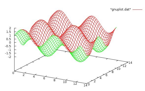
A special case is tests for Laplace Equation
ΔU = 0 or ∇2U = 0 or Uxx(x,y) + Uyy(x,y) = 0 or
∂2U/∂x2 + ∂2U/∂y2 = 0
Many known solutions and thus Dirichlet boundary conditions
for test cases are known:
k>0 is any constant
U(x,y)=k
U(x,y)=k*x
U(x,y)=k*y
U(x,y)=k*x*y
U(x,y)=k*x^2 - k*y^2
U(x,y)=sin(k*x)*sinh(k*y)
U(x,y)=sin(k*x)*cosh(k*y)
U(x,y)=cos(k*x)*sinh(k*y)
U(x,y)=cos(k*x)*cosh(k*y)
U(x,y)=sin(k*x)*exp( k*y)
U(x,y)=sin(k*x)*exp(-k*y)
U(x,y)=cos(k*x)*exp( k*y)
U(x,y)=cos(k*x)*exp(-k*y)
r=sqrt(x^2+y^2)
th=atan2(y,x) -Pi..Pi principal value is
U(x,y)=r^k * sin(k*th) discontinuous along negative X axis
using atan2 in 0..2Pi wrong!
causes discontinuous derivative along positive X axis
When the number of degrees of freedom gets large, the size of
the matrix for the system of simultaneous equations may get
larger than acceptable for your computer.
For example a four dimensional PDE with 10 DOF in each dimension
has 10^4 = 10,000 DOF. The non sparse simultaneous equations
would require at least 10,000 by 10,000 entries, 10^8 times
8 bytes = 0.8GB.
Much larger PDE's, need to be solved.
A sparse matrix stores only the non zero entries.
A system of simultaneous equations does not have a unique
solution if any row is all zeros, thus a sparse structure
has at least one entry of each row. Then in each row,
the column index and value are stored for the non zero
values. Typical spare data structures use a singly linked
list for each row, keeping the column index in increasing
numerical order.
Optimized code is typically written for inserting and
adding entries, solving simultaneous equations, vector
times matrix multiplication and a few other operations.
For various languages, the sparse packages are shown with
the initial test programs and several PDE solutions.
"C" implementation of sparse
"C" source code sparse.c
"C" header file sparse.c
"C" test code test_sparse.c
test output test_sparse_c.out
"C" more test code test1_sparse.c
test output test1_sparse_c.out
simple conversion to sparse_abc.c
output of sparse_abc_c.out
"C" source code pde44_sparse.c
test_output pde44_sparse_c.out
Ada implementation of sparse
For subscripts starting with zero
Ada source code sparse.adb
Ada package specification sparse.ads
Ada test code test_sparse.adb
test output test_sparse_ada.out
For subscripts starting with one
Ada source code sparse1.adb
Ada package specification sparse1.ads
Ada test code test_sparse1.adb
test output test_sparse1_ada.out
simple conversion to sparse_abc.adb
output of sparse_abc_ada.out
Ada source code pde44_sparse.adb
test_output pde44_sparse_ada.out
Java implementation of sparse
Java source code sparse.java
Java test code test_sparse.java
test output test_sparse_java.out
simple conversion to sparse_abc.java
output of sparse_abc_java.out
Java source code pde44_sparse.java
test_output pde44_sparse_java.out
Fortran implementation of sparse
For subscripts starting with zero
Fortran source code sparse.f90
Fortran test code test_sparse.f90
test output test_sparse_f90.out
For subscripts starting with one
Fortran source code sparse1.f90
Fortran test code test_sparse1.f90
test output test_sparse1_f90.out
Fortran source code pde44_sparse.f90
test_output pde44_sparse_f90.out
Some of the most difficult to solve PDE's have an
"order" greater than one. These are nonlinear PDE's.
A specific problem, challenge if you prefer, is the
possibility of "non physical solutions" and
"bifurcating solutions" in addition to no possible solution.
A small change in the boundary conditions or a different
starting vector for the nonlinear solver can produce
different results with no way of knowing the result is
ambiguous.
A PDE having any product or ratio of U, Ux, Uxx, etc.
is nonlinear. In two dimensions Uxx*Uxx, Uxx*UYY, etc.
Several nonlinear PDE of interest are:
Second order, third degree:
U^2 U'' + 2 U U' + 3U = f(x)
Reciprocal nonlinear:
D U' - E(x) U'/U^2 - F U'' = f(x)
An example that can handle up to third degree nonlinear systems of
equations is shown by using a Newton iteration based on the inverse
of the Jacobian:
x_next = x_prev - J^-1 * ( A * x_prev - Y)
Java nonlinear
simeq_newton5.java basic solver
test_simeq_newton5.java test program
test_simeq_newton5_java.out test_output
on four test cases (automatic adjusting heuristic used)
A linear PDE using conventional Finite Element Method, FEM, works:
source code fem_nl11_la.java
output fem_nl11_la_java.out
A nonlinear PDE using conventional FEM does not work.
source code fem_nl12_la.java
output fem_nl12_la_java.out
(very similar, nonlinear, fails)
Discretization works on nonlinear PDE's:
source code pde_nl21.java
output pde_nl21_java.out
source code pde_nl22.java
output pde_nl22_java.out
solver simeq_newton5.java
Ada nonlinear PDE
simeq_newton5.adb basic solver
test_simeq_newton5.adb test program
test_simeq_newton5_ada.out test_output
on five test cases (automatic adjusting heuristic used)
hard coded nonlinear coefficients, non unique solution
source code pde_nl13.adb
output pde_nl13_ada.out
solver simeq_newton5.adb
automated computation of nonlinear coefficients, still non unique solution
source code pde_nl13a.adb
output pde_nl13a_ada.out
solver simeq_newton5.adb
More examples with many checks:
source code pde_nl21.adb
output pde_nl21_ada.out
source code pde_nl22.adb
output pde_nl22_ada.out
Third order PDE in 3 dimensions with 3rd degree nonlinearity.
Demonstrates use of least square fit of boundary as an
initial guess to solve nonlinear system of equations.
See Lecture 4 for lsfit.ads, lsfit.adb
source code pde_nl33.adb
output pde_nl33_ada.out
Python3 nonlinear PDE
simeq_newton5.py3 basic solver
test_simeq_newton5.py3 test program
test_simeq_newton5_py3.out test_output
test_pde_nl.py3 test program
test_pde_nl_py3.out test_output
C nonlinear
source code pde_nl13.c
output pde_nl13_c.out
solver simeq_newton5.c
header simeq_newton5.h
difficulties
The nonlinear PDE can not be solved by simple application
of Finite Element Method, covered in lecture 32.
For example, the above nonlinear PDE is not solved by:
source code fem_checknl_la.c
output fem_checknl_la_c.out
Using discretization with a nonlinear solver, such as simeq_newton5,
works accurately and efficiently.
Kuramoto-Sivashinsky nonlinear
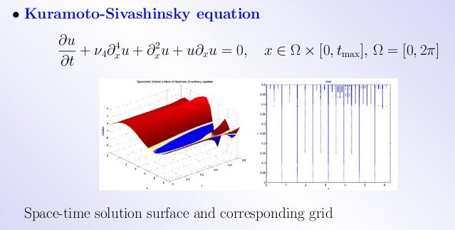 There seem to be many variations of the Kuramoto-Sivashinsky
non linear, fourth order PDE, depending on the physical problem.
I have seen in various reference papers:
Ut + Uxxxx + Uxx + 1/2 (Ux)^2 = 0 mainly variations in the last term, and
∂U(x,t)/∂t + ∂^4 U(x,t)/∂x^4 + ∂^2 U(x,t)/∂x^2 -(∂U(x,t)/∂x)^2 = 0
In the figure below, read h as U, read y as t.
There seem to be many variations of the Kuramoto-Sivashinsky
non linear, fourth order PDE, depending on the physical problem.
I have seen in various reference papers:
Ut + Uxxxx + Uxx + 1/2 (Ux)^2 = 0 mainly variations in the last term, and
∂U(x,t)/∂t + ∂^4 U(x,t)/∂x^4 + ∂^2 U(x,t)/∂x^2 -(∂U(x,t)/∂x)^2 = 0
In the figure below, read h as U, read y as t.
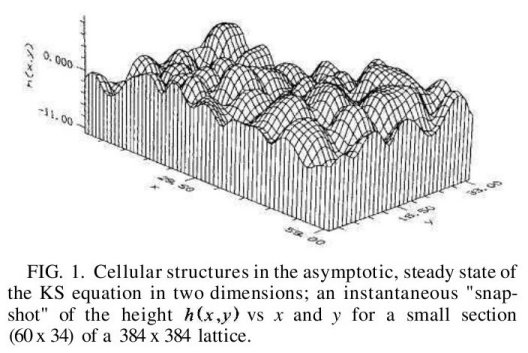 For nonlinear PDE to be solved by solving a system of equations,
the simultaneous equations are non linear.
To solve a system of nonlinear equations reasonably efficiently,
use a Jacobian matrix and an iterative solution and adaptive
solver such as simeq_newton5, available in a few languages.
For nonlinear PDE to be solved by solving a system of equations,
the simultaneous equations are non linear.
To solve a system of nonlinear equations reasonably efficiently,
use a Jacobian matrix and an iterative solution and adaptive
solver such as simeq_newton5, available in a few languages.
Two dimensional nonlinear PDE
Solve (Uxx(x,y) + Uyy(x,y))^2 = F(x,y)
expand to
Uxx(x,y)*Uxx(x,y) + 2*Uxx(x,y)*Uyy(x,y) + Uyy(x,y)*Uyy(x,y) = F(x,y)
For pde_nl22 (Uxx(x,y)+Uyy(x,y))^2 = F(x,y)
2D grid for partial differential equation grid nx by ny
Unknown U, given boundary B, for this case nx=7, ny=6.
Zero based indexing, xmin=0.0, xmax=0.6, ymin=0.0, ymax=0.4
Does not need to be uniform, this grid has hx=0.1, hy=0.08
Uk=S(i,ii)=(i-1)*ny+(ii-1)
0.0 0.1 0.2 0.3 0.4 0.5 0.6 X
ii +------+------+------+------+------+------+------+ Y
5 | B0,5 : B1,5 : B2,5 : B3,5 : B4,5 : B5,5 | B6,5 |
+------+======+======+======+======+======+------+ 0.40
4 | B0,4 | U3 | U7 | U11 | U15 | U19 | B6,4 |
+------+------+------+------+------+------+------+ 0.32
3 | B0,3 | U2 | U6 | U10 | U14 | U18 | B6,3 |
+------+------+------+------+------+------+------+ 0.24
2 | B0,2 | U1 | U5 | U9 | U13 | U17 | B6,2 |
+------+------+------+------+------+------+------+ 0.16
1 | B0,1 | U0 | U4 | U8 | U12 | U16 | B6,1 |
+------+======+======+======+======+======+------+ 0.08
0 | B0,0 : B1,0 : B2,0 : B3,0 : B4,0 : B5,0 : B6.0 |
+------+------+------+------+------+------+------+ 0.0
0 1 2 3 4 5 6 i
Source code for solution using C, with output and debugging output
source code pde_nl22.c
output pde_nl22_c.out
output with debugging pde_nl22_c.ckout
files needed to compile and link
source code simeq_newton3.h
source code simeq_newton3.c
source code deriv.h
source code deriv.c
source code invert.h
source code invert.c
Source code for solution using Java, with output and debugging output
source code pde_nl22c,java
output pde_nl22c_java.out
output with debugging pde_nl22c_java.ckout
files needed to build
source code simeq_newton3.java
source code nuderiv.java
source code invert.java
Maple used to generate analytic solution for building test case.
Maple analytic solution pde_nl22_mws.out
Note approximate quadratic convergence to solution, from output files:
solve non linear equations A * U = F
simeq_newton3 running
simeq_newton3 itr=0, prev=1e+12, residual=71032.2
simeq_newton3 itr=1, prev=71032.2, residual=17757.5
simeq_newton3 itr=2, prev=17757.5, residual=4438.85
simeq_newton3 itr=3, prev=4438.85, residual=1109.29
simeq_newton3 itr=4, prev=1109.29, residual=276.986
simeq_newton3 itr=5, prev=276.986, residual=68.9598
simeq_newton3 itr=6, prev=68.9598, residual=17.0073
simeq_newton3 itr=7, prev=17.0073, residual=4.08366
simeq_newton3 itr=8, prev=4.08366, residual=0.906544
simeq_newton3 itr=9, prev=0.906544, residual=0.164953
simeq_newton3 itr=10, prev=0.164953, residual=0.0220222
simeq_newton3 itr=11, prev=0.0220222, residual=0.00342033
simeq_newton3 itr=12, prev=0.00342033, residual=0.000446783
simeq_newton3 finished
Now we attack solving the PDE on multicore and multiprocessor
computer architectures.
The basic concept is to use worker task to do the parallel
computation and a master control task, the main procedure,
to keep the workers synchronized. These examples, in several
languages, use the barrier method of synchronization.
The first example is converting fem_check44_la.adb to
a parallel version. We developed psimeq, parallel simultaneous
equations solver in lecture 3b
Thus we need to choose the number of processors, NP, to pass
to psimeq.
Then we need to parallelize the longest computation, creating
the stiffness matrix, as covered in lecture 32
Care must be taken to insure no worker tasks set any variable that
might by modified by any other worker task or the master task.
Parallelizing Ada, FEM example
fem_check44_pla.adb
fem_check44_pla_ada.out
The other files needed to compile and execute include:
psimeq.ada
laphi.ads
laphi.adb
gaulegf.adb
real_arrays.ads
real_arrays.adb
Ada barrier software
Parallelizing Java, FEM example
The first example is converting fem_check44_la.adb to
a parallel version. We developed psimeq, parallel simultaneous
equations solver in lecture 3b
Thus we need to choose the number of processors, NP, to pass
to psimeq.
Then we need to parallelize the longest computation, creating
the stiffness matrix, as covered in lecture 32
Care must be taken to insure no worker tasks set any variable that
might by modified by any other worker task or the master task.
fem_check44_pla.java
fem_check44_pla_java.out
Now we attack solving the PDE on multicore and multiprocessor
computer architectures using multiple precision arithmetic.
Many examples use GMP, Gnu Multiple Precision.
The basic concept is to use worker task to do the parallel
computation and a master control task, the main procedure,
to keep the workers synchronized. These examples, in several
languages, use the barrier method of synchronization.
Using pthreads and gmp to solve large systems of
simultaneous equations.
mpf_tsimeq.h
mpf_tsimeq.c
time_mpf_tsimeqb.c
time_mpf_tsimeqb.out
A sample of using top -H
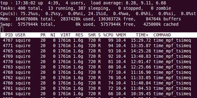
A brief introduction to the "Finite Element Method" FEM,
using the Galerkin Method is galerkin.pdf
There are entire books on FEM and this just covers one small view.
Examples demonstrating the above galerkin.pdf
are shown below. The examples are for Degree 1 (linear), Order 1 through 4,
Dimension 1 through 7. Several programming languages are shown for
some of the examples. Results were close to the same in time and
accuracy for various languages.
The first two examples use three methods of integration:
Adaptive, Newton-Coates and Gauss-Legendre.
For these cases Gauss-Legendre was best.
fem_checke_la.c first order, one dimension
fem_checke_la_c.out output with debug print
fem_checke_la.adb first order, one dimension
fem_checke_la_ada.out output with debug print
fem_checke_la.f90 first order, one dimension
fem_checke_la_f90.out output with debug print
fem_check4th_la.c fourth order, one dimension
fem_check4th_la_c.out output with debug print
fem_check4th_la.adb fourth order, one dimension
fem_check4th_la_ada.out output with debug print
fem_check4th_la.f90 fourth order, one dimension
fem_check4th_la_f90.out output with debug print
fem_check22_la.c second order, two dimension
fem_check22_la_c.out output with debug print
fem_check22_la.adb second order, two dimension
fem_check22_la_ada.out output with debug print
fem_check22_la.f90 second order, two dimension
fem_check22_la_f90.out output with debug print
fem_check22_la.java second order, two dimension
fem_check22_la_java.out output with debug print
with a small study of grid size and integration order, solution with exp(g(x,y))
fem_check22e_la.java second order, two dimension
fem_check22e_la_java.out output with debug print
fem_check_abc_la.c second order, two dimension
fem_check_abc_la_c.out output with debug print
abc_la.h problem definition
abc_la.c problem definition
fem_check_abc_la.adb second order, two dimension
fem_check_abc_la_ada.out output with debug print
abc_la.ads problem definition
abc_la.adb problem definition
fem_check_abc_la.f90 second order, two dimension
fem_check_abc_la_f90.out output with debug print
abc_la.f90 problem definition
fem_check33_la.c third order, three dimension
fem_check33_la_c.out output with debug print
fem_check33_la.f90 third order, three dimension
fem_check33_la_f90.out output with debug print
fem_check33_la.adb third order, three dimension
fem_check33_la_ada.out output with debug print
fem_check33_la.java third order, three dimension
fem_check33_la_java.out output with debug print
npx=3 gave error 10^-12, npx=4 gave error 10^-13 little better for bigger npx
fem_check44_la.c fourth order, four dimension
fem_check44_la_c.out output with debug print
fem_check44_la.f90 fourth order, four dimension
fem_check44_la_f90.out output with debug print
fem_check44_la.adb fourth order, four dimension
fem_check44_la_ada.out output with debug print
fem_check44_la.java fourth order, four dimension
fem_check44_la_java.out output with debug print
fem_check47h_la.c fourth order, seven dimension
fem_check47h_la_c.out output with debug print
fem_check47h_la.java fourth order, seven dimension
fem_check47h_la_java.out output with debug print
In getting ready for this lecture, I have tried many versions of FEM.
The "historic" or classic methods used very low order orthogonal
polynomials and a piecewise linear approach. The trade-off I found was
the time to solve of very large systems of equations vs the time for
numerical quadrature for a much smaller system of equations.
Another trade-off was the complexity of coding the special cases
that arise in piecewise linear approximations. There are many
published tables and formulas for the general case using many
geometric shapes. What is generally missing is the tables and
formulas for the cells next to the boundary.
I found that developing a library routine for the various derivatives
of phi and using high order Lagrange polynomials led to minimizing
programming errors. Each library routine must, of course, be
thoroughly tested. Here are my Lagrange phi routines and tests.
laphi.h "C" header file
laphi.c code through 4th derivative
test_laphi.c numeric test
test_laphi_c.out test output
plot_laphi.c plot test
laphi.ads Ada package specification
laphi.adb code through 4th derivative
test_laphi.adb numeric test
test_laphi_ada.out test output
laphi.f90 module through 4th derivative
test_laphi.f90 numeric test
test_laphi_f90.out test output
laphi.java class through 4th derivative
test_laphi.java numeric test
test_laphi_java.out test output
Other files, that are needed by some examples above:
aquade.ads Ada package specification
aquade.adb tailored adaptive quadrature
gaulegf.adb Gauss-Legendre quadrature
simeq.adb solve simultaneous equations
real_arrays.ads Ada package specification
real_arrays.adb types Real, Real_Vector, Real_Matrix
aquad3.h "C" header file
aquad3.c tailored adaptive quadrature
aquad3e.f90 tailored adaptive quadrature
gaulegf.f90 Gauss-Legendre quadrature
simeq.f90 solve simultaneous equations
gaulegf.java Gauss-Legendre quadrature
simeq.java solve simultaneous equations
A simple PDE and solution, well lots of code:
ΔU = Uxx + Uyy = F(x,y) = 2Π2*(cos(2Π*x)*sin2(Π*y) + sin2(Π*x)*cos(2Π*y))
Known solution U(x,y) =sin2(Π*x)*sin2(Π*y)
Using utility routines .c and .h above
fem22_la.c source code
fem22_la_c.out output
fem22_la_c.dat computed solution for plot
fem22_la_c.sh gnuplot driver
fem22_la_c.plot gnuplot control
fem22_la_c.png the result plot
 Run with Makefile entry:
fem22_la_c.out: fem22_la.c simeq.h simeq.c gaulegf.h gaulegf.c laphi.h laphi.c
gcc -o fem22_la fem22_la.c simeq.c gaulegf.c laphi.c -lm
fem22_la > fem22_la_c.out
rm -f fem22_la
./fem22_la_c.sh # gnuplot uses fem22_la_c.plot fem22_la_c.dat
Run with Makefile entry:
fem22_la_c.out: fem22_la.c simeq.h simeq.c gaulegf.h gaulegf.c laphi.h laphi.c
gcc -o fem22_la fem22_la.c simeq.c gaulegf.c laphi.c -lm
fem22_la > fem22_la_c.out
rm -f fem22_la
./fem22_la_c.sh # gnuplot uses fem22_la_c.plot fem22_la_c.dat
A brief introduction to the "Finite Element Method" FEM,
using triangles or tetrahedrons rather than a uniform grid.
The previous Galerkin Method galerkin.pdf
applies with some changes.
There are entire books on FEM and this just covers one small view.
Examples are shown below. The examples are for Degree 1 (linear),
with Order 1 through 4,
Dimension 2 (triangle) and Dimension 3 (tetrahedron)
Some specialty stuff that may be used later:
affine_map_tri.txt triangle mapping
test_affine_map.c test program
test_affine_map.out output
test_affine_map2.c test program
test_affine_map2.out output
test_affine_map.html Maple solution
test_affine_map.mw Maple worksheet
Given a set of coordinates and a boundary path, generate a set of
triangles that cover the interior. Four sets are shown below:
The programs are triangle.c and showme.c run using commands:
triangle A.poly generates file A.1.poly A.1.node A.1.ele
showme -p A.1.poly plots boundary, click on ele to plot triangles
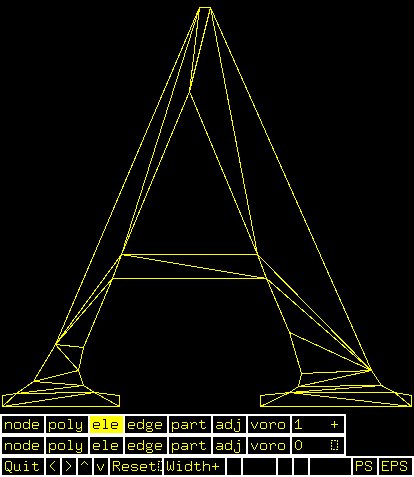 A.poly initial input (simpler ones follow)
A.1.poly generated by program triangle
A.1.ele generated by program triangle
A.1.node generated by program triangle
triangle -D -a0.01 -q30 -p B.poly generates B.1.*
showme -p B.1.poly wait for menus at bottom, click on ele
A.poly initial input (simpler ones follow)
A.1.poly generated by program triangle
A.1.ele generated by program triangle
A.1.node generated by program triangle
triangle -D -a0.01 -q30 -p B.poly generates B.1.*
showme -p B.1.poly wait for menus at bottom, click on ele
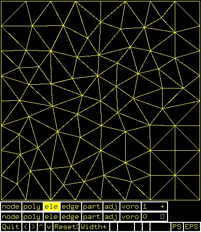 B.poly initial input (square)
B.1.poly generated by program triangle
B.1.ele generated by program triangle
B.1.node generated by program triangle
triangle -D -a0.1 -q30 -p C.poly generates C.1.*
showme -p C.1.poly wait for menus at bottom, click on ele
B.poly initial input (square)
B.1.poly generated by program triangle
B.1.ele generated by program triangle
B.1.node generated by program triangle
triangle -D -a0.1 -q30 -p C.poly generates C.1.*
showme -p C.1.poly wait for menus at bottom, click on ele
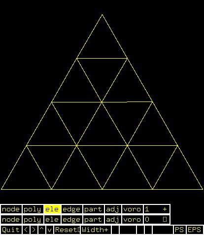 C.poly initial input (triangle)
C.1.poly generated by program triangle
C.1.ele generated by program triangle
C.1.node generated by program triangle
triangle -D -a2.0 -q45 -p D.poly generates D.1.*
showme -p D.1.poly wait for menus at bottom, click on ele
C.poly initial input (triangle)
C.1.poly generated by program triangle
C.1.ele generated by program triangle
C.1.node generated by program triangle
triangle -D -a2.0 -q45 -p D.poly generates D.1.*
showme -p D.1.poly wait for menus at bottom, click on ele
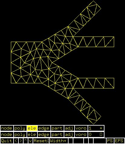 D.poly initial input (channels)
D.1.poly generated by program triangle
D.1.ele generated by program triangle
D.1.node generated by program triangle
triangle.c source code
triangle.help documentation
triangle.readme sample commands
triangle.README README
showme.c source code
note: the C.1.node C.1.ele C.1.poly can be used for fem_check below
C.coord C.tri C.bound by deleting sequence numbers
and extra trailing stuff
D.poly initial input (channels)
D.1.poly generated by program triangle
D.1.ele generated by program triangle
D.1.node generated by program triangle
triangle.c source code
triangle.help documentation
triangle.readme sample commands
triangle.README README
showme.c source code
note: the C.1.node C.1.ele C.1.poly can be used for fem_check below
C.coord C.tri C.bound by deleting sequence numbers
and extra trailing stuff
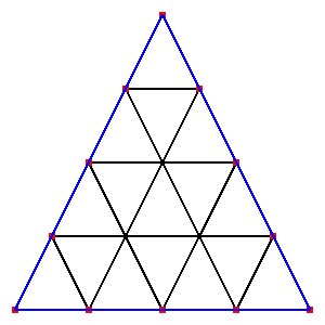 C.coord from C.1.node
C.tri from C.1.ele
C.bound from C.1.poly
plot_fem_tri.c plots .coord,.tri,.bound
C.coord from C.1.node
C.tri from C.1.ele
C.bound from C.1.poly
plot_fem_tri.c plots .coord,.tri,.bound
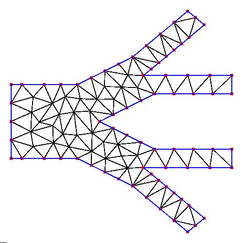 D.coord from D.1.node
D.tri from D.1.ele
D.bound from D.1.poly
The most basic geometry and several triangle splits:
22_t.coord 3 triangles, 4 vertices
22_t.tri 3 boundary, 1 free
22_t.bound
Any FEM group can be split, every triangle becomes 4 triangles that
are one fourth the area and congruent to the original triangles.
This cuts "h" the longest edge in half and should improve accuracy,
up to some limit, at the cost of longer execution time.
do_tri_split.c
22_ts.coord 12 triangles, 10 vertices
22_ts.tri 6 boundary, 4 free
22_ts.bound
22_tss.coord 48 triangles, 31 vertices
22_tss.tri 12 boundary, 19 free
22_tss.bound
The D.poly from above as original, split once, split again
Circles can be split into triangles:
D.coord from D.1.node
D.tri from D.1.ele
D.bound from D.1.poly
The most basic geometry and several triangle splits:
22_t.coord 3 triangles, 4 vertices
22_t.tri 3 boundary, 1 free
22_t.bound
Any FEM group can be split, every triangle becomes 4 triangles that
are one fourth the area and congruent to the original triangles.
This cuts "h" the longest edge in half and should improve accuracy,
up to some limit, at the cost of longer execution time.
do_tri_split.c
22_ts.coord 12 triangles, 10 vertices
22_ts.tri 6 boundary, 4 free
22_ts.bound
22_tss.coord 48 triangles, 31 vertices
22_tss.tri 12 boundary, 19 free
22_tss.bound
The D.poly from above as original, split once, split again
Circles can be split into triangles:
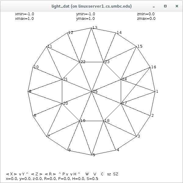 circle_tri.coord
circle_tri.tri
circle_tri.bound
circle_tri.dat
Circles can be grided:
circle_tri.coord
circle_tri.tri
circle_tri.bound
circle_tri.dat
Circles can be grided:
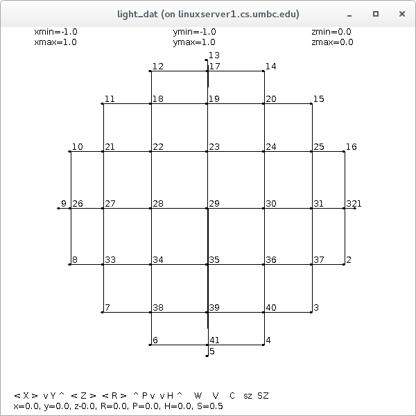 circle_grid.dat
circle_grid.java
Program files that produces the images above:
tri_input.java
tri_split.java
test_tri_split.java
circle_tri.java
The first example of FEM on triangles is a first order in two dimensions.
fem_check21_tri.c source code
fem_check21_tri.out output 22_tri
fem_check21_tria.out output 22_t
fem_check21_tri_C.out output C
additional files needed for execution of the above:
phi_tri.h source code
phi_tri.c source code
phi_tri_cm.h source code
phi_tri_cm.c source code
phi_tri_pts.h source code
phi_tri_pts.c source code
A similar example in Java of FEM on triangles is a first order in two dimensions.
This is an improved version from fem_check21
fem_check21a_tri.java source code
fem_check21a_tri22_t.out output
fem_check21a_tri22_ts.out output
fem_check21a_tri22_tss.out output
additional files needed for execution of the above:
triquad.java source code
simeq.java source code
the test for accuracy of triquad.java are:
test_triquad.java source code
test_triquad.out results, see last two sets
the test for accuracy of triquad_int.c are:
triquad_int.c source code
test_triquad_int.c test code
In order to understand the complexity of the code,
the following figures show one vertex, V1, that is a
part of three triangles, T1, T2 and T3.
For vertex V1 there are three test functions, phi1, phi2 and phi3,
represented by blue for the phi1, yellow for phi2 and red for phi3.
These test functions are shown as linear "hat" functions, yet could
be higher order test functions.
circle_grid.dat
circle_grid.java
Program files that produces the images above:
tri_input.java
tri_split.java
test_tri_split.java
circle_tri.java
The first example of FEM on triangles is a first order in two dimensions.
fem_check21_tri.c source code
fem_check21_tri.out output 22_tri
fem_check21_tria.out output 22_t
fem_check21_tri_C.out output C
additional files needed for execution of the above:
phi_tri.h source code
phi_tri.c source code
phi_tri_cm.h source code
phi_tri_cm.c source code
phi_tri_pts.h source code
phi_tri_pts.c source code
A similar example in Java of FEM on triangles is a first order in two dimensions.
This is an improved version from fem_check21
fem_check21a_tri.java source code
fem_check21a_tri22_t.out output
fem_check21a_tri22_ts.out output
fem_check21a_tri22_tss.out output
additional files needed for execution of the above:
triquad.java source code
simeq.java source code
the test for accuracy of triquad.java are:
test_triquad.java source code
test_triquad.out results, see last two sets
the test for accuracy of triquad_int.c are:
triquad_int.c source code
test_triquad_int.c test code
In order to understand the complexity of the code,
the following figures show one vertex, V1, that is a
part of three triangles, T1, T2 and T3.
For vertex V1 there are three test functions, phi1, phi2 and phi3,
represented by blue for the phi1, yellow for phi2 and red for phi3.
These test functions are shown as linear "hat" functions, yet could
be higher order test functions.
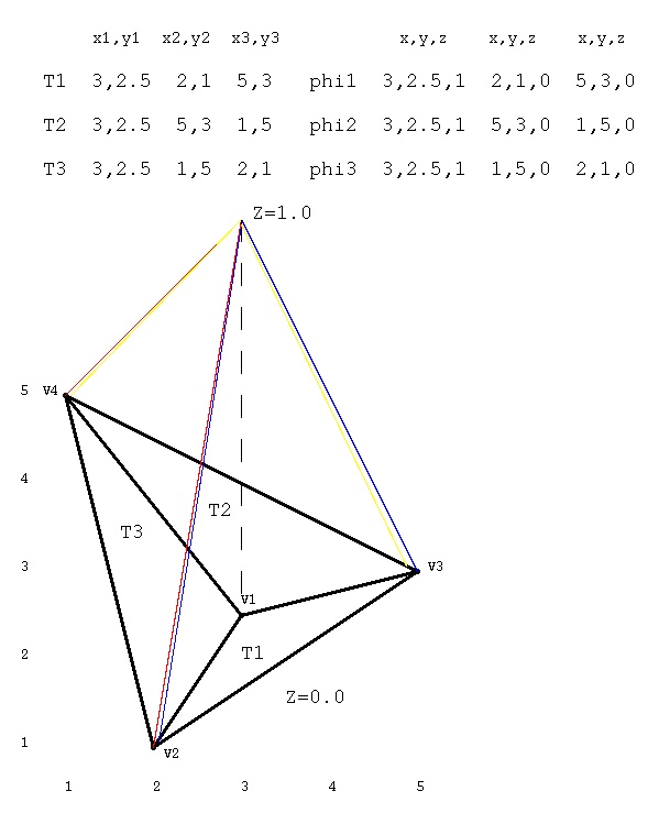 The triangles are in the plane Z=0.0.
All three test functions are at Z=1.0 above the vertex of interest,
V1. All three test functions are at Z=0.0 for all other vertices
in the triangles that include vertex V1.
Looking down on the triangles, the three test functions can be seen
to cover the area of the three triangles T1, T2 and T3 with functions
phi1, phi2 and phi3.
The triangles are in the plane Z=0.0.
All three test functions are at Z=1.0 above the vertex of interest,
V1. All three test functions are at Z=0.0 for all other vertices
in the triangles that include vertex V1.
Looking down on the triangles, the three test functions can be seen
to cover the area of the three triangles T1, T2 and T3 with functions
phi1, phi2 and phi3.
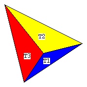 The equation
 is, in the general case, computed by numerical quadrature
of the linear operator, L, with the dependent variable and
its derivatives replaced by a test function and corresponding
derivatives of the test function.
For the triangulation shown above and for the first equation,
for vertex V1, there are three numerical quadratures that
are summed to get the integral as shown.
The first region, omega is T1 and the test function is phi1.
The second region, omega is T2 and the test function is phi2.
The third region, omega is T3 and the test function is phi3.
In the integral equation, the omega is the sum of T1, T2 and T3.
In the integral equation, the symbol φ1 is phi1 for T1,
phi2 for T2 and phi3 for T3.
In general, the global stiffness matrix is constructed by
processing one triangle at a time. The the integral shown
above accumulates the sum as the three triangles containing
the vertex V1 are processed in some order. In general there
will be more than three triangles that contain a vertex.
A general outline of FEM for triangles is presented in
femtri.pdf
is, in the general case, computed by numerical quadrature
of the linear operator, L, with the dependent variable and
its derivatives replaced by a test function and corresponding
derivatives of the test function.
For the triangulation shown above and for the first equation,
for vertex V1, there are three numerical quadratures that
are summed to get the integral as shown.
The first region, omega is T1 and the test function is phi1.
The second region, omega is T2 and the test function is phi2.
The third region, omega is T3 and the test function is phi3.
In the integral equation, the omega is the sum of T1, T2 and T3.
In the integral equation, the symbol φ1 is phi1 for T1,
phi2 for T2 and phi3 for T3.
In general, the global stiffness matrix is constructed by
processing one triangle at a time. The the integral shown
above accumulates the sum as the three triangles containing
the vertex V1 are processed in some order. In general there
will be more than three triangles that contain a vertex.
A general outline of FEM for triangles is presented in
femtri.pdf
Second Order Basis Functions
There is a large variety of basis functions, test functions,
or "phi" functions using FEM terminology. For triangles,
a family of second order, 6 point, functions is:
tri_basis.h source code
tri_basis.c source code
test_tri_basis.c test code
test_tri_basis.out test output
plot_tri_basis.c plotting code
plot_tri_basis2.c plotting code
plot is dynamic with motion, run it yourself, type "n" for next function
Scaled Lobatto shape functions may be used in conjunction with
other basis functions.
lobatto_shape.h source code
lobatto_shape.c source code
plot_lobatto.c source code
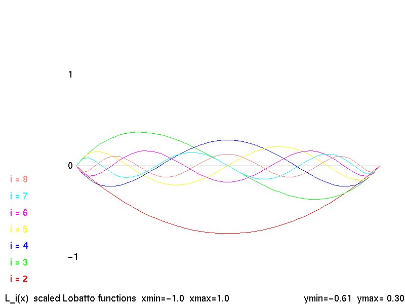 Lobatto k-2 shape functions
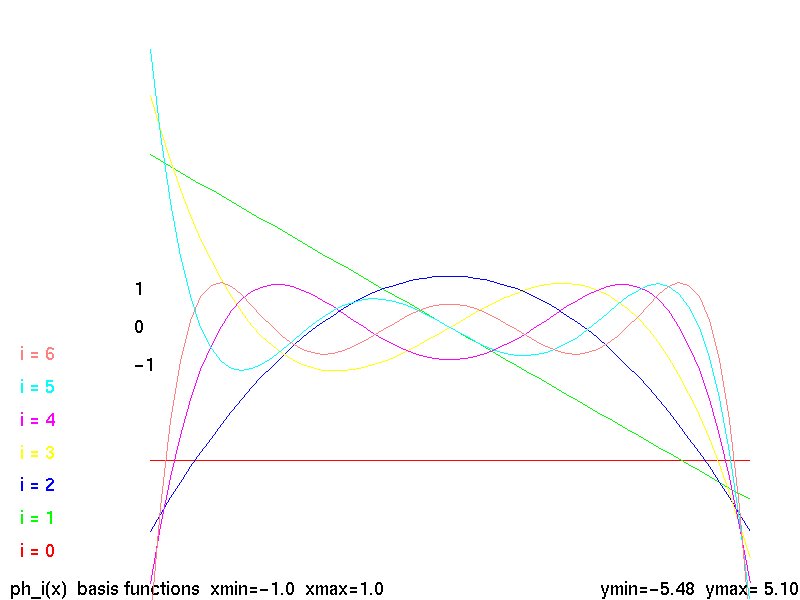 basis functions
Discretization of Triangular Grids
A very different method than FEM to solve a subset of
FEM triangle PDE's, uses discretization of a group
of points, subset of the vertices, and simultaneous
equations to get a solution.
The primary technique is the non uniform discretization of
a set of points, given in two dimensions:
nuderiv2dg.java source code
test_nuderiv2dg_tri.java test code
test_nuderiv2dg_tri_java.out test output
test_nuderiv2dg2_tri.java test code
test_nuderiv2dg2_tri_java.out test output
test_nuderiv2dg3_tri.java test code
test_nuderiv2dg3_tri_java.out test output
pde_nuderiv2dg_tri.java pde code
pde_nuderiv2dg_tri_java.out pde output
simeq.java utility class
A weaker form, note missing 'g' for general, that requires independent
points is:
nuderiv2d.java source code
test_nuderiv2d.java test code
test_nuderiv2d_java.out test output
Tetrahedrons for three dimensions
Then, for three dimensions, we need tetrahedrons in place of triangles.
test_split_tetra.c test code
test_split_tetra.out test output
plot_split_tetra.c plot program
tetra_split.java utility program
test_tet_split.java test program
plot with light_dat.java source
heapsort.java source needed by light_dat
sphere_tri1.dat sphere as 8 triangles
sphere_tet1.dat sphere as 8 tetrahedrons
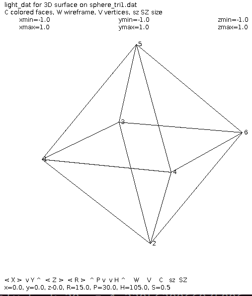
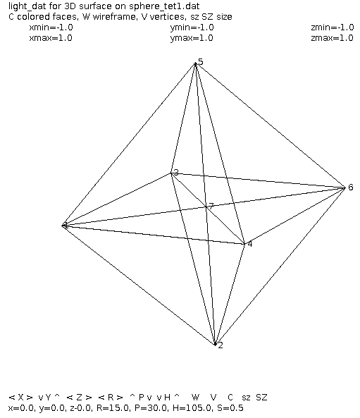 sphere_tri2.dat sphere as 48 triangles
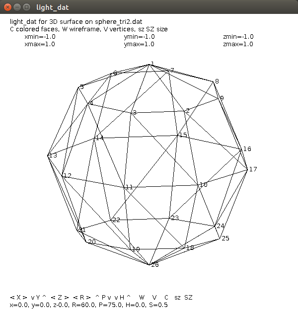
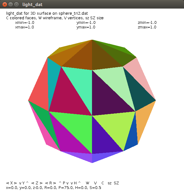 tetra_split.dat tetrahedron split
 cube_tetra.tet cube split into tetrahedrons 4 points
cube_tetra.dat cube split into tetrahedrons 4 triangle surfaces
cube_tetra.tet cube split into tetrahedrons 4 points
cube_tetra.dat cube split into tetrahedrons 4 triangle surfaces

High order basis functions and integration
pde2sin_la.adb code, sin(x-y) 0 to 4Pi
pde2sin_la_ada.out output
pde2sin4_la.dat data for plot

Challenging Modeling and Simulation
Solving Maxwell's equations for electric fields can be
very challenging. I have not been able to numerically
compute the discharge pattern shown below.
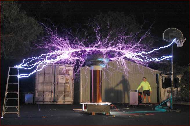 Maxwell's Equations
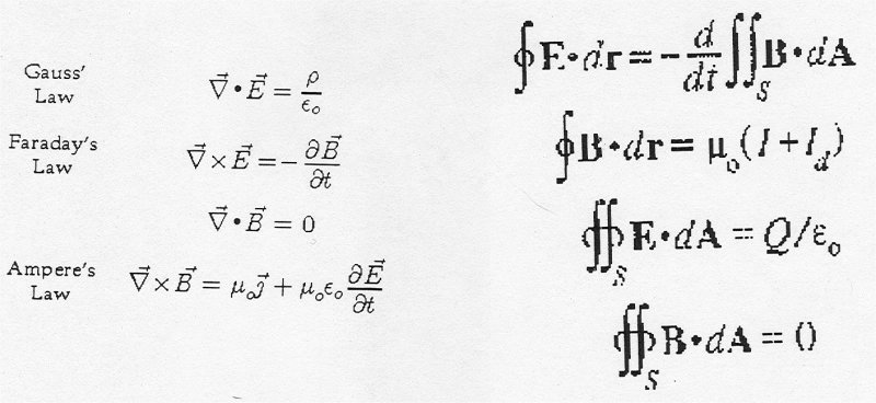
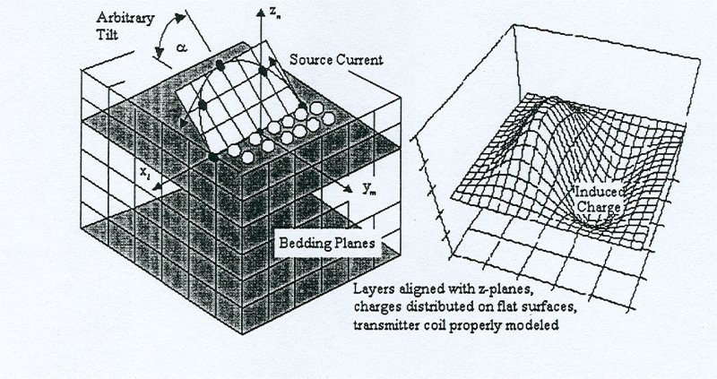 The numerical solution of Maxwell's Equations for electro-magnetic
fields may use a large four dimensional array with dimensions
X, Y, Z, T. Three spatial dimensions and time.
The numerical solution of Maxwell's Equations for electro-magnetic
fields may use a large four dimensional array with dimensions
X, Y, Z, T. Three spatial dimensions and time.
Phi functions for triangles.
Using basic Lagrange polynomials to get a value 1.0 at
the vertex of interest and a value of 0.0 at the other
two vertices.
A "C" implementation is shown by:
phi_tril.c
phi_tril.h
A Matlab implementation with resulting plots is:
phi_tril.m
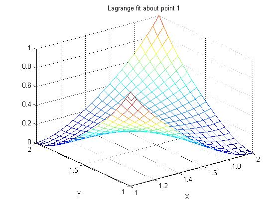
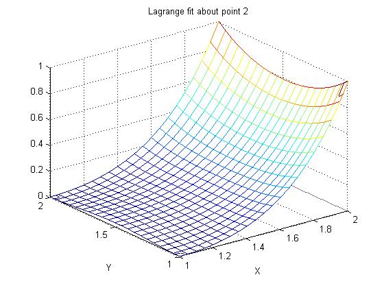
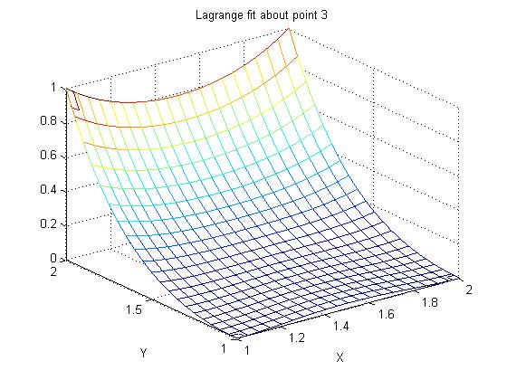
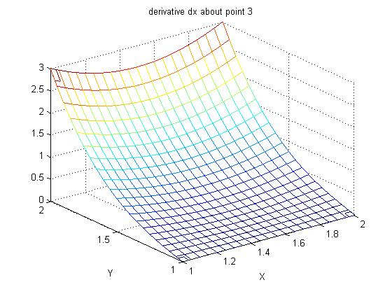
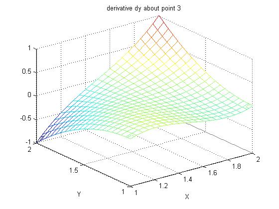
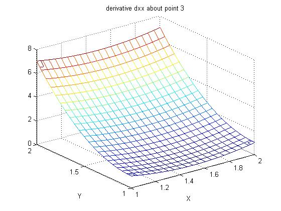
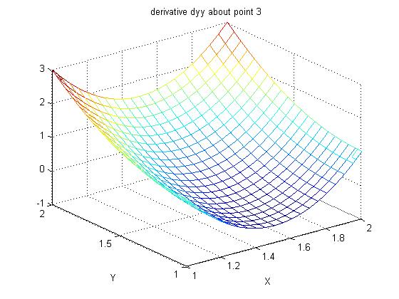
Recent update.
There are many file formats that may be of interest.
Collected here are a tiny fraction of what is available.
Search the web for code to read and convert formats.
Adapt existing code to the language of your choice.
AVS UCD data
AVS UCD data format
UCD cyl1.inp demonstrating boundary conditions
This file defines a rectangular duct with a cylinder inside.
The Dirichlet and Neumann boundary conditions are specified
as well as the geometry.
cyl1.inp boundary definition
plot_ucd.c for plotting 3D UCD boundary
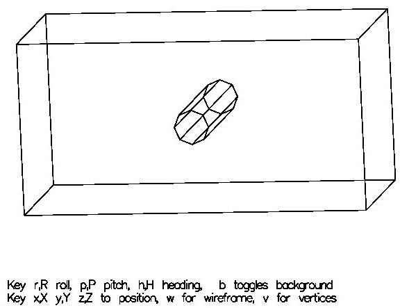
Extending UCD data to 4 dimensions
Without changing the basic UCD format,
the 4th coordinate can be provided along with
Dirichlet and Neumann boundary conditions.
pde_ucd4.inp 4D geometry
Source code to read UCD format
read_ucd.h C++ header
read_ucd.cc C++ code
test_read_ucd.cc C++ test
ucd1.inp test input data
ucd1.out test output results
ucd2.inp test input data
ucd2.out test output results
Ada Language implementation, including use in a PDE
pde_read_ucd.ads Ada package spec
pde_read_ucd.adb Ada package body
test_pde_read_ucd.adb test
test_pde_read_abc_ucd_ada.out test results
pde_process_ucd.ads Ada package spec
pde_process_ucd.adb Ada package body
test_pde_process_ucd.adb test
test_pde_process_abc_ucd_ada.out test results
make_abc_ucd.adb make abc_ucd.inp
abc_ucd.inp UCD file
abc_ucd.ads PDE definition spec
abc_ucd.adb PDE definition body
pde_abc_eq_ucd.adb PDE solver
pde_abc_eq_ucd_ada.out solution
UCD file with color, mechanical properties, ranges
The UCD File Format is very versatile.
This file is just a demonstration of the flexibility.
# ucd1.inp Sample AVS UCD File
#
9 8 1 3 5 9 nodes, 8 cells, 1 node data, 3 cell data, 5 model
1 0.000 0.000 1.000 Node coordinates
2 1.000 0.000 1.000
3 1.000 1.000 1.000
4 0.000 1.000 1.000
5 0.000 0.000 0.000
6 1.000 0.000 0.000
7 1.000 1.000 0.000
8 0.000 1.000 0.000
9 0.500 0.600 0.707
1 1 hex 1 2 3 4 5 6 7 8 cell id, material id, cell type, cell node numbers
2 1 tri 1 3 4
3 1 pt 1
4 1 tet 2 3 4 5
5 2 line 7 9
6 2 quad 2 4 6 8
7 2 prism 1 2 3 6 7 8
8 2 pyr 2 3 4 5 6
1 1 number of node components, size of each component
stress, lb/in**2 Component name, units name
1 4999.9999 Data value for each node component
2 18749.9999
3 37500.0000
4 56250.0000
5 74999.9999
6 93750.0001
7 107500.0003
8 5000.0001
9 5001.0000
1 3 number of cell components, size of each component
RGB, cell color component name, units name
2 1.0 0.0 0.0 Data value for each cell component
1 0.0 1.0 0.0 (Do not have to be in order, some may require order)
3 0.0 0.0 1.0
4 1.0 1.0 0.0
5 1.0 0.0 1.0
6 0.0 1.0 1.0
7 0.5 0.5 0.5
8 0.7 0.7 0.7
2 2 2 number of model components, size of each component
limits, min/max min/max component name, value description
range, min/max min/max component name, value description
1 -1.0 1.0 -1.0 1.0
2 -1.2 1.2 -1.3 1.3
3 -1.5 1.5 -1.6 1.6
4 -1.9 2.0 -2.0 1.9
5 -2.0 2.0 -2.0 2.0
Lecture 35, Navier Stokes Airfoil Simulation
Basically, this is a study to see if the 1933 wind tunnel
measurements of airfoils for coefficient of lift CL and
coefficient of drag CD can be reproduced by computer
simulation.
Airfoil 0015
Testing formulas for 0015 airfoil
rotate_prime.java
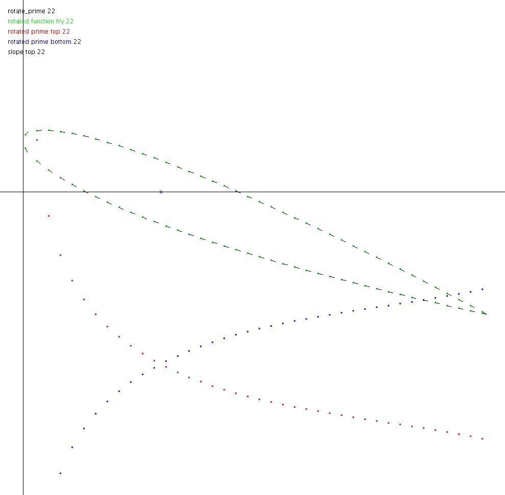 Create data file for airfoil at a specific angle and grid:
w0015grid.java
Build a PDE analysis grid around the airfoil:
w0015vert.java
Create data file for airfoil at a specific angle and grid:
w0015grid.java
Build a PDE analysis grid around the airfoil:
w0015vert.java
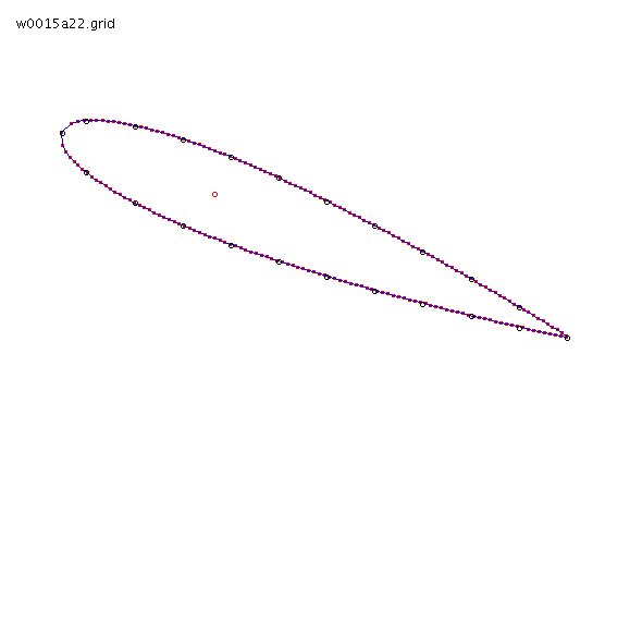
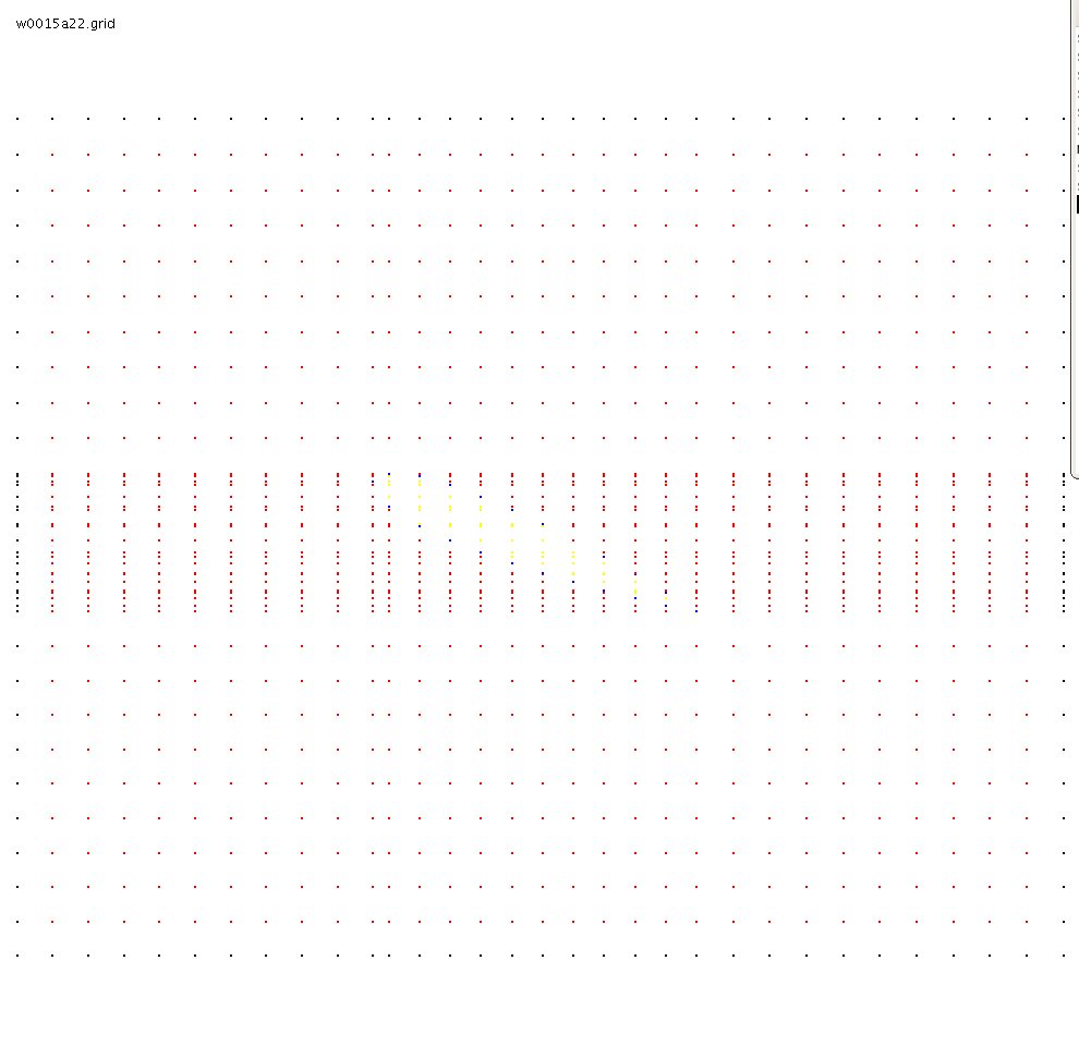 w0015grid_java.out
w0015a22.grid
w0015vert_java.out
w0015grid_java.out
w0015a22.grid
w0015vert_java.out
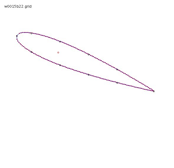
 w0015b22_grid_java.out
w0015b22.grid
w0015b22_vert_java.out
w0015b22_grid_java.out
w0015b22.grid
w0015b22_vert_java.out
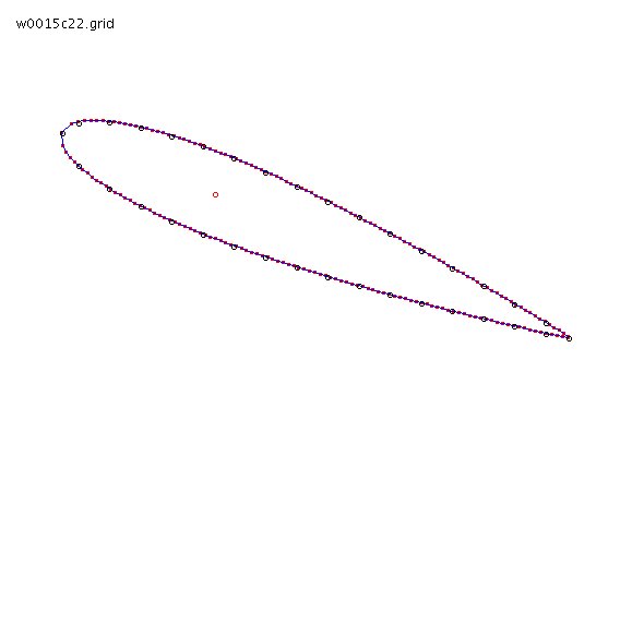
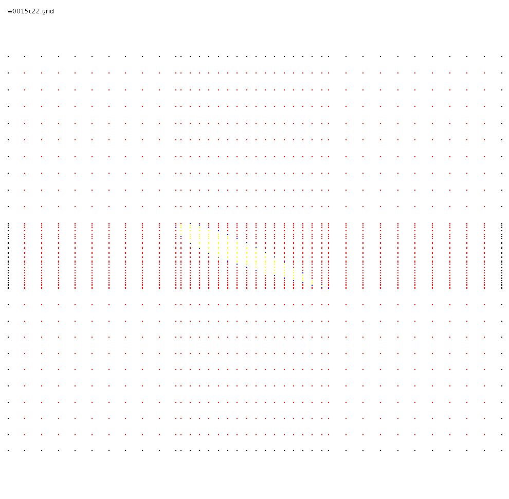 w0015c22_grid_java.out
w0015c22.grid
w0015c22_vert_java.out
w0015c22_grid_java.out
w0015c22.grid
w0015c22_vert_java.out
 w0015b00.grid
w0015b00_vert_java.out
References:
NACA-460 1933 78 airfoils
NACA-824 1945 Airfoil Summary
w0015b00.grid
w0015b00_vert_java.out
References:
NACA-460 1933 78 airfoils
NACA-824 1945 Airfoil Summary
Lecture 36, Some special PDE's
From "A Collection of 2D Elliptic Problems for Testing
Adaptive Algorithms" by William F. Mitchell
1. Solutions of the form
U(x,y)=2^4p x^p (x-1)^p y^p (y-1)^p for p=4
PDE Uxx(x,y) + Uyy(x,y) = f(x,y)
boundary unit square
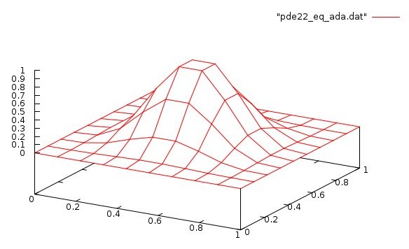 pde22_eq.adb
pde22_eq_ada.out
pde22_eq_ada.dat
pde22_eq_ada.plot
pde22_eq_ada.sh
pde22_eq.c
pde22_eq_c.out
pde22_eq_c.dat
pde22_eq_c.plot
pde22_eq_c.sh
pde22_eq.java
pde22_eq_java.out
pde22_eq_java.dat
pde22_eq_java.plot
pde22_eq_java.sh
pde22_eq.f90
pde22_eq_f90.out
pde22_eq_f90.dat
pde22_eq_f90.plot
pde22_eq_f90.sh
pde22_eq.adb
pde22_eq_ada.out
pde22_eq_ada.dat
pde22_eq_ada.plot
pde22_eq_ada.sh
pde22_eq.c
pde22_eq_c.out
pde22_eq_c.dat
pde22_eq_c.plot
pde22_eq_c.sh
pde22_eq.java
pde22_eq_java.out
pde22_eq_java.dat
pde22_eq_java.plot
pde22_eq_java.sh
pde22_eq.f90
pde22_eq_f90.out
pde22_eq_f90.dat
pde22_eq_f90.plot
pde22_eq_f90.sh
Then U(x,y)=2^4p x^p (x-1)^p y^p (y-1)^p for p=10
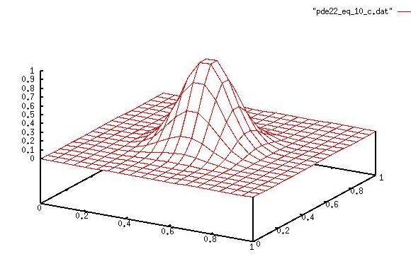 pde22_eq_10.c
pde22_eq_10_c.out
pde22_eq_10_c.dat
pde22_eq_10_c.plot
pde22_eq_10_c.sh
pde22_eq_10.c
pde22_eq_10_c.out
pde22_eq_10_c.dat
pde22_eq_10_c.plot
pde22_eq_10_c.sh
Then U(x,y)=4*(x-1)*(x-3)*(x-3)*(y-1)*(y-3)*(y-3) p=9
 pde22b_eq.java source code
simeq.java source code
rderiv.java source code
pde22b_eq_java.out
pde22b_eq_java.dat
pde22b_eq_java.plot
pde22b_eq_java.sh
pde22b_eq.java source code
simeq.java source code
rderiv.java source code
pde22b_eq_java.out
pde22b_eq_java.dat
pde22b_eq_java.plot
pde22b_eq_java.sh
Then U(x,y)=5*(x*x+x)*(y*y+y) p=9
 pde22d_eq.java
pde22d_eq_java.out
pde22d_eq_java.dat
pde22d_eq_java.plot
pde22d_eq_java.sh
pde22d_eq.java
pde22d_eq_java.out
pde22d_eq_java.dat
pde22d_eq_java.plot
pde22d_eq_java.sh
2. Solutions of the form
alpha = Pi/omega
r = sqrt(x^2+y^2)
theta = atan2(y,x) 0..2Pi
U(x,y)=r^alpha * sin(alpha*theta)
PDE Uxx(x,y) + Uyy(x,y) = 0
boundary x -1..1, y -1..1
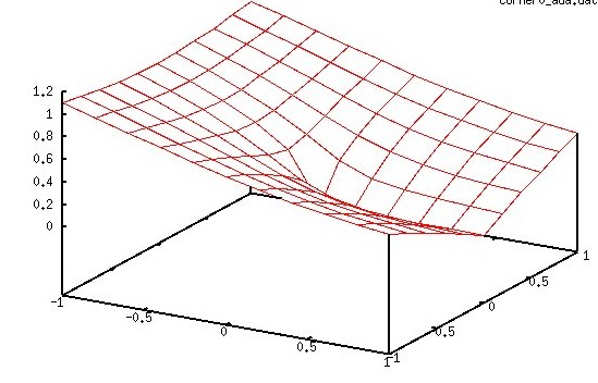 Exact solution
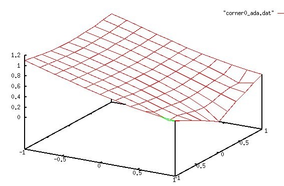 nx=11, ny=11 uniformly spaced, computed solution
corner0.adb
corner0_ada.out
corner0_ada.dat
corner0_ada.plot
corner0_ada.sh
corner0.c
corner0_c.out
corner0_c.dat
corner0_c.plot
corner0_c.sh
corner0.java
corner0_java.out
corner0_java.dat
corner0_java.plot
corner0_java.sh
corner0.f90
corner0_f90.out
corner0_f90.dat
corner0_f90.plot
corner0_f90.sh
nx=11, ny=11 uniformly spaced, computed solution
corner0.adb
corner0_ada.out
corner0_ada.dat
corner0_ada.plot
corner0_ada.sh
corner0.c
corner0_c.out
corner0_c.dat
corner0_c.plot
corner0_c.sh
corner0.java
corner0_java.out
corner0_java.dat
corner0_java.plot
corner0_java.sh
corner0.f90
corner0_f90.out
corner0_f90.dat
corner0_f90.plot
corner0_f90.sh
Makefile and other files for programs listed above
Makefile_spde
nuderiv.adb
inverse.adb
simeq.adb
real_arrays.ads
real_arrays.adb
nuderiv.c
inverse.c
simeq.c
mpf_nuderivd.c
mpf_inverse.c
nuderiv.java
inverse.java
simeq.java
nuderiv.f90
inverse.f90
simeq.f90
Have gnuplot installed to get plots.
Have gnat installed for .adb
Have gcc installed for .c
Have Java installed for .java
Have gfortran installed for .f90
PDE for Turbulence and Diffusion
pde_turbulence.pdf
diffusion_equation
Generic_scalar_transport_equation
Unusual geometries and using all differentials
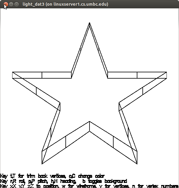
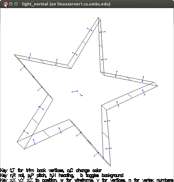 The red dot is the positive direction of the normal to the surface.
Plotted with light_normal.c to be sure all surfaces have normal
pointing out. This is needed to be able to determine if a
point is inside the volume and process Neumann boundary conditions.
poly43.txt
All 4th order derivatives in 3 dimensions.
pde_star3t.java
Used in pde_star3t.java.
The red dot is the positive direction of the normal to the surface.
Plotted with light_normal.c to be sure all surfaces have normal
pointing out. This is needed to be able to determine if a
point is inside the volume and process Neumann boundary conditions.
poly43.txt
All 4th order derivatives in 3 dimensions.
pde_star3t.java
Used in pde_star3t.java.
Lecture 36a, Special discretization, non uniform
We have arbitrarily scattered boundary points and DOF.
No structure is provided. The problem is to discretize
and build a system of equations, solve the equations,
and determine the values at the DOF.
Simple 1D demonstration
check_nuderiv.c just 6 points
check_nuderiv_c.out check solution
check_nuderiv.java just 6 points
check_nuderiv_java.out check solution
So far, only for 2D and 3D geometry, yet could be generalized.
The basic problem is avoiding singular matrices.
The worse case of arbitrarily scattered points is
when they are uniformly spaced.
The basic non uniform discretization:
nuderiv2d.c use all points
nuderiv2d.h
test_nuderiv2d.c
test_nuderiv2d_c.out
nuderiv2dg.c use good points, less singular
nuderiv2dg.h
test_nuderiv2dg.c
test_nuderiv2dg_c.out
nuderiv2d.java use all points
test_nuderiv2d.java
test_nuderiv2d_java.out
nuderiv2dg.java use good points, less singular
test_nuderiv2dg.java
test_nuderiv2dg_java.out
Now a corner geometry
test_nuderiv2dgc.c
test_nuderiv2dgc_c.out
The basic 3D non uniform discretization:
nuderiv3d.c use all points
nuderiv3d.h
test_nuderiv3d.c
test_nuderiv3d_c.out
nuderiv3dg.c use good points, less singular
nuderiv3dg.h
test_nuderiv3dg.c
test_nuderiv3dg_c.out
nuderiv3dg.java use good points, less singular
test_nuderiv3dg.java
test_nuderiv3dg_java.out
Applying non uniform discretization to a PDE
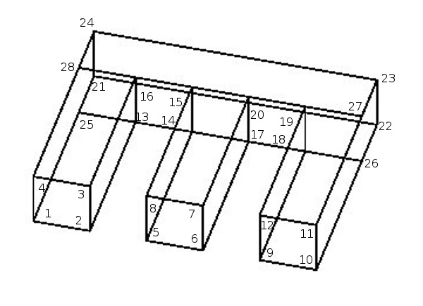 blivet.inp zero based, regular
blivet_nr.inp non regular
pde_blivet.c
pde_blivet_c.out
pde_blivet_nr_c.out
pde_blivet.java
pde_blivet_java.out
pde_blivet_nr_java.out
blivet.inp zero based, regular
blivet_nr.inp non regular
pde_blivet.c
pde_blivet_c.out
pde_blivet_nr_c.out
pde_blivet.java
pde_blivet_java.out
pde_blivet_nr_java.out
Lecture 37, various utility routines
Permutations, Combinations, Heapsort
Some various utility routines that may be used for applications
or generating tests.
Generating all permutations of a vector
permute.h
permute.c
test_permute.c
test_permute_c.out
permute.ads
permute.adb
test_permute.adb
test_permute_ada.out
permute.java
test_permute.java
test_permute_java.out
permute2.java
permute2_java.out
super_perm.txt super permutations
super_perm.shtml super permutations
Generating Combinations of N things taken M at a time
combinations.h
combinations.c
test_combinations.c
test_combinations_c.out
combinations.ads
combinations.adb
test_combinations.adb
test_combinations_ada.out
combinations.java
test_combinations.java
test_combinations_java.out
Heap Sort a vector, get sort indices, multi dimensions
heapsort.h
heapsort.c
test_heapsort.c int, double, char
test_heapsort_c.out
test2_heapsort.c on struct
test2_heapsort_c.out
heap_sort_2.ads
heap_sort_2.adb
test_heap_sort_2.adb
test_heap_sort_2_ada.out
heapsort.java
test_heapsort.java
test_heapsort_java.out
get_close.java
test_get_close.java
test_get_close_java.out
test_sort.java source code
test_sort_java.out output
time_test_sort.java source code
time(test_sort_java.out output
test_sort.py3 source code
test_sort_py3.out output
time_test_sort.py3 source code
time_test_sort_py3.out output
A version of the traveling salesman program, tsp.
Once in a while, the heuristic solution O(n^2) comes out
the same as the NP Complete solution.
Every run gets different random numbers.
tsp.c
tsp.out
Lecture 38, Open Tutorial on LaTeX
You can prepare high quality math and engineering
papers using LaTeX, pronounced lah tech.
This is not intended to cover all or even most of LaTeX.
You will prepare a LaTeX file foo.tex
running LaTeX
On UMBC GL machines you have several options to get output:
latex foo.tex
latex foo.tex # this is needed for TOC, bibliography, etc
dvips -o foo.ps foo.dvi # compiling produces a .dvi and other files
lpr foo.ps # print high quality PostScript
# your browser can view foo.ps, lower quality print
ps2pdfwr foo.ps foo.pdf # optional to also produce a .pdf
pdflatex foo.tex # generate a .pdf
acroread foo.pdf # use acroread to view and print
evince foo.pdf # use evince to view and print
# your browser can view and print foo.pdf
and, many other auxiliary programs are available.
Use your favorite editor to create foo.tex
Best on-line reference is:
http://en.wikibooks.org/wiki/LaTeX
Getting LaTeX on your computer
Linux: sudo apt-get install texlive
MacOSX: get mactex
Windows: get protext or miktex
First example
Here is a simple, complete, .tex file
hello.tex
hello.ps
hello.pdf
% hello.tex absolute minimum to get output
\documentclass[12pt]{letter} % could be paper, article, report, book, slides ...
\begin{document} % start of document
Hello world from LaTeX.
\end{document} % end of document, nothing after this line
The Makefile commands to generate hello.ps and hello.pdef are:
latex hello.tex
latex hello.tex
dvips -o hello.ps hello.dvi
ps2pdfwr hello.ps hello.pdf
Note some syntax "\" and "{ }"
"\" starts a command, there are many.
You can define new commands to save on typing.
More commands can be brought in from packages
"{ }" are for grouping or enclosing. Usually REQUIRED!
e.g. \frac {numerator equation} {denominator equation}
Generally, arbitrary nesting is allowed, just use
lots of { { {} {} } { } }
one or mode spaces is a space.
carriage return and tab are a space.
lines automatically formatted unless you interfere
No semicolons at end of lines or statements
Printing equations
equation.tex
equation.ps
 % equation.tex just a few samples
\documentclass[12pt]{article}
\begin{document} % start of document
For subscript use underscore
$A_1 \; \; A_i \; \; A_{i,j} $ % \; for more spaces
For power, superscript use hat % $ your equation $
$x^2 \; \; x^{p+q} \; \; x^{y^z} $
${n \choose k} = \frac{n!}{k!(n-k!)}$
$z = \sqrt {x^2 + y^2}$
\[ \int _{i=0} ^{\infty} \frac {1}{{(x+1)}^2} dx \]
\( \sum _{j=1} ^{10} A_j \)
\end{document} % end of document, nothing after this line
% equation.tex just a few samples
\documentclass[12pt]{article}
\begin{document} % start of document
For subscript use underscore
$A_1 \; \; A_i \; \; A_{i,j} $ % \; for more spaces
For power, superscript use hat % $ your equation $
$x^2 \; \; x^{p+q} \; \; x^{y^z} $
${n \choose k} = \frac{n!}{k!(n-k!)}$
$z = \sqrt {x^2 + y^2}$
\[ \int _{i=0} ^{\infty} \frac {1}{{(x+1)}^2} dx \]
\( \sum _{j=1} ^{10} A_j \)
\end{document} % end of document, nothing after this line
printing matrices and vectors
Using \matrix
pdemat.tex
pdemat.ps
pdemat.pdf
% pdemat.tex
\documentclass[11pt,fleqn]{article} % preamble follows
\setlength{\textheight}{8.5in}
\setlength{\topmargin}{0.5in}
\setlength{\textwidth}{6.5in}
\setlength{\headheight}{0.0in}
\setlength{\headsep}{0.0in}
\setlength{\oddsidemargin}{0in}
\newcommand{\LL}{\mit L}
\begin{document} % start of document
System of simultaneous equations that are too wide for paper
$$\left| \matrix{ \int_{\Omega} \LL \left( \phi_1(x,y) \right) \phi_1(x,y) dx \, dy \
\int_{\Omega} \LL \left( \phi_2(x,y) \right) \phi_1(x,y) dx \, dy \
\ldots \
\int_{\Omega} \LL \left( \phi_{nxy}(x,y) \right) \phi_1(x,y) dx \, dy \cr
\int_{\Omega} \LL \left( \phi_1(x,y) \right) \phi_2(x,y) dx \, dy \
\int_{\Omega} \LL \left( \phi_2(x,y) \right) \phi_2(x,y) dx \, dy \
\ldots \
\int_{\Omega} \LL \left( \phi_{nxy}(x,y) \right) \phi_2(x,y) dx \, dy \cr
\ldots \cr
\int_{\Omega} \LL \left( \phi_1(x,y) \right) \phi_{nxy}(x,y) dx \, dy \
\int_{\Omega} \LL \left( \phi_2(x,y) \right) \phi_{nxy}(x,y) dx \, dy \
\ldots \
\int_{\Omega} \LL \left( \phi_{nxy}(x,y) \right) \phi_{nxy}(x,y) dx \, dy \cr
} \right|
\times
$$
$$ \left| \matrix{ U_1 \cr U_2 \cr \ldots \cr U_{nxy} \cr } \right|
=
\left| \matrix{ \int_{\Omega} f(x,y) \phi_1(x,y) dx \, dy \cr
\int_{\Omega} f(x,y) \phi_2(x,y) dx \, dy \cr
\ldots \cr
\int_{\Omega} f(x,y) \phi_{nxy}(x,y) dx \, dy \cr } \right|
$$
\end{document} % end of document, nothing after this line
Drawings that have a lot of math symbols
put(x,y){\
Lecture 39, Tutorial on numerical solution of differential equations
The goal of this lecture is to have the student understand how
to numerically compute the solution of a differential equation.
The numerical solution will be computed by a computer program.
Almost any computer language can be used to compute the numerical
solution of differental equations. Various languages will be
used as examples. Much of the notation will be more computer
programming oriented than mathematical.
This lecture starts with very basic concepts and defines the notation
that will be used.
Expect terms to be defined close to the terms first usage.
We start with ordinary differential equations and then cover
partial differential equations.
An ordinary differential equation has exactly one independent
variable, typically x .
A partial differential equation has more than one independent
variable, typically x,y x,y,z x,y,z,t etc.
understanding derivatives
From a numerical point of view, the derivative of
a function is the slope at a specific value for the
independent variable.
The second derivative is just the derivative of
the first derivative of a function.
Note*** first a polynomial, then the sine
we know from Calculus:
U(x) = sin(x)
U'(x) d/dx sin(x) = cos(x) the first derivative od sine x is cosine x
U''(x) d/dx cos(x) = -sin(x) the second derivative of sine x is -sine x
U'''(x) d/dx -sin(x) = -cos(x) the third derivative of sine x is -cosine x
Look at the plot of sin(x) and its derivatives.
Note the slope of each curve at each point, is the derivative
plotted below it. A few are highlighted by red, blue and
green dots.

notation for ordinary differential equations
f(x) A function of x, typically any function of one independent variable.
x^3 + 7 x^2 + 5 x + 4 is a polynomial function of x,
x cubed plus 7 times x squared plus 5 times x plus 4 .
sin(x) a function of x that computes the sine of x .
All trignometric functions will use x in radians.
y=f(x) an equation, some times written y = f(x);
y'(x)=3 x^2 + 14 x + 5; y(0)=4;
A differential equation with an initial condition.
The analytic solution is f(x) the polynomial above.
Given y=f(x) , y'(x) is the notation for taking
the first derivative of f(x),
also written as d/dx f(x) or d f(x)/dx .
Typically we are given a starting and ending value
for which the numerical solution is needed.
The result may be a table of x,y values and
often a graphical plot of the solution.
y''''(x)-y(x)=0; y(0)=0; y'(0)=1; y''(0)=0; y'''(0)=-1;
A fourth order differential equation with initial conditions.
We will see later why four initial conditions are
needed in order to compute the numerical solution.
We know the analytic solution is f(x)=sin(x);
yet we will see that we must be careful of errors
in computing the numerical solution.
a(x)*y'' + b(x)*y' + c(x) = 0 is a second order ordinary
differential equation. The three functions a(x),
b(x), and c(x) must be known and programmable.
In general functions will appear more than
constants in differential equations.
notation for partial differential equations
f(x,y,z) a function of three independent variables.
2*x*y^2*z + 4*x^2*z^2 + 3*y
a polynomial in three variables
2 times x times y squared times z plus
4 times x squared times z squared plus 3 time y
U(x,y,z) will be the numerical solution of a partial differential
equation giving values of f(x,y,z) in a specified three
dimensional region.
Ux(x,y,z) or just Ux if the independent variables are obvious,
is the first derivative with respect to x of f(x,y,z) .
Uxx is the second derivative with respect to x of f(x,y,z)
Uxy is the first derivative with respect to x of f(x,y,z)=Ux
then the first derivative with respect to y of Ux.
Uxyyz is the first derivative with respect to x, then the
second derivative with respect to y, then the first
derivative with respect to z.
Uxxx + a(x,y,z)*Uyyz + b(x,y,z)*Uz = c(x,y,z);
Is a partial differential equation.
In order to numerically solve this equation we need
the three functions a(x,y,z), b(x,y,z) and c(x,y,z)
to be specified and we must be able to code them
in the programming language we wish to use to
compute the numerical solution.
Typically this type of partial differential equation
has a closed three dimensional volume, called the
boundary, where the solution must be computed.
Enough values of the function f(x,y,z) must be
given, typically on the boundary, to have a
unique solution defined. These values are known
as Dirchilet boundary values. Derivative values
may also be provided on the boundary, these are
known as Neumann boundary values.
required conditions
In order to compute a unique numerical solution we need:
1) The function f that is the solution must be continuous
and continuously differentiable in and on the boundary.
(Solving for discontinuous results, such as shock waves
is beyond the scope of this tutorial.)
2) There must be enough boundary values to make the
solution unique. At least one Dirichilet value must
be given and possibly some number of Neumann values.
3) The boundary must be given. For this tutorial we
cover only one closed boundary with no internal "holes".
4) The coordinate system is assumed Cartesian unless
otherwise specified, Polar, Cylindrical, Spherical,
Elipsoidal, or other.
numerically solving our first ordinary differential equation
Lecture 40, unique numerical solution of differential equations
The goal of this lecture is to show the long development
cycle of a unique numerical solution of a partial differential
equation in the domain of an arbitrary 3D closed polyhedra with
Dirchilet boundary conditions at the vertices.
The development included using several file formats to define
the closed polyhedra and the developing code to be sure that
the polyhedra was really closed. There may be one or more
polyhedra "hole" completely inside the outer closed polyhedra.
Just determining the "refinement", the location of internal
points where the solution is to be computed was needed.
Previous solutions have used FEM, finite element method and
various forms of discretization. Basically building a system
of linear equations containing the internal points and then
solving the system of linear equations to get the solution
at each point. The unique method that came about during this
development is to solve for each internal point, DOF, degree
of freedom serially, independent of any other internal point.
This also makes the solution easily parallizable to any
number of processores.
The intuition came from studying one internal point that
seemed to be surrounded by a randomly scattered bunch of
vertices. Oh! If I could compute the derivatives in the
PDE at that point based on boundary vertices with known
Dirchilet values, the only unknown is the solution at
that internal point. Yes I can. My object of interest
was a Medieval Spiked Flail, the surface was a bunch
of points created out of tetrahedrons.
Now, to the formal development, specifically for three
dimensions, although it does generalize. Also limited
to fourth order derivatives, although that could be
increased.
The series of Makefile runs
sphere_div.c data generator
spike.dat polyhedra
format changer .dat to .inp UCD
spike.inp polyhedra UCD format
datread.h .dat format read 3D figure,
datread.c into working arrays
test_datread.c test read and closed polyhedra
test_datread_c.out spike.dat OK
pde_read_ucd.h .inp format read 3D figure,
pde_read_ucd.c etc., into working arrays
test_pde_read_ucd.c read and print data
test_pde_read_spike_c.out
test_pde_inside3_ucd.c point in polyhedra
test_pde_inside3_ucd_c.out point in polyhedra tested
nuderiv3dg.h derivative from random points
nuderiv3dg.c up to 4th order in 3 variables
test_nuderiv3dg.c test every call
test_nuderiv3dg_c.out all OK
lsfit.h multidimensional polynomial fit,
lsfit.c fit from random points
test_lsfit7.c sample test
test_lsfit7_c.out sample output
simeq.h solve simultameous equations
simeq.c solve simultameous equations
test_simeq.c simple test
test_simeq_c.out OK
point_in_poly.h determine if a point
point_in_poly.c is in polygon or polyhedra
test_point_in_poly.c test
test_point_in_poly_c.out results
pde_spike.c solve 4th order PDE on spike.inp
pde_spike_c.out test results
Lecture 41, Numerically solving AC circuits
Spice is one of a number of electrical circuit simulation programs.
Our UMBC computers have a version called ngspice installed.
This is an example of a transient analysis, computed by integration
in small time steps. Similar to our rocket simulation.
Spice circuit input
capdio.cir voltage multiplier ngspice -b capdio.cir > capdio.out
VS 99 0 AC 10 SIN(0VOFF 10VPEAK 1KHZ)
R1 99 98 1
C1 98 1 1UF
C2 0 2 1UF
C3 1 3 1UF
C4 2 4 1UF
C5 3 5 1UF
C6 4 6 1UF
D1 0 1
D2 1 2
D3 2 3
D4 3 4
D5 4 5
D6 5 6
.TRAN 100US 50MS
.print tran V(1) V(2) V(3) V(4) V(5) V(6)
.plot tran V(1) V(2) V(3) V(4) V(5) V(6)
.end
The schematic diagram with node numbers is:
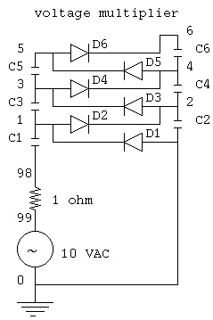 The simulation with time step of 100 microseconds
for 0.01 seconds shows the voltage buildup at
the six nodes 1, 2, 3, 4, 5, 6 in the circuit.
The simulation with time step of 100 microseconds
for 0.01 seconds shows the voltage buildup at
the six nodes 1, 2, 3, 4, 5, 6 in the circuit.
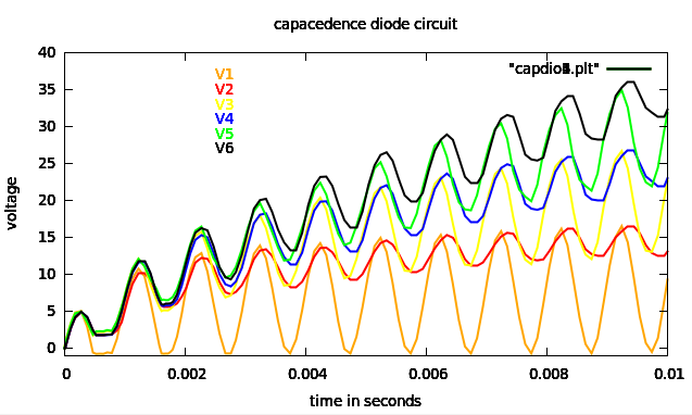 Running the simulation to 0.04 seconds shows
stable voltage at node 6.
Running the simulation to 0.04 seconds shows
stable voltage at node 6.
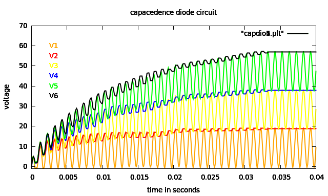 Another type of Spice simulation is to simulate
a circuit at a series of frequencies. Type AC.
After setup of a matrix, solve simultaneous
equations to compute results.
Spice circuit input
ac.cir ac tuned circuit ngspice -b ac.cir > ac.out
I 0 1 ac 1000.0
R1 0 1 0.001
R2 1 2 1000.0
R3 1 3 1000.0
R4 1 4 1000.0
R5 1 5 1000.0
C1 2 0 0.0000001591549431
L1 3 0 0.1591549431
C2 4 0 0.0000001591549431
L2 4 0 0.1591549431
C3 5 6 0.0000001591549431
L3 6 0 0.1591549431
*F1 10.0 100000.0 10.0
.ac DEC 20 100 10k $ 100Hz to 10kHz, 20 points per decade
.print AC V(1) V(2) V(3) V(4) V(5)
.plot AC V(2) V(3) V(4) V(5)
.end
Another type of Spice simulation is to simulate
a circuit at a series of frequencies. Type AC.
After setup of a matrix, solve simultaneous
equations to compute results.
Spice circuit input
ac.cir ac tuned circuit ngspice -b ac.cir > ac.out
I 0 1 ac 1000.0
R1 0 1 0.001
R2 1 2 1000.0
R3 1 3 1000.0
R4 1 4 1000.0
R5 1 5 1000.0
C1 2 0 0.0000001591549431
L1 3 0 0.1591549431
C2 4 0 0.0000001591549431
L2 4 0 0.1591549431
C3 5 6 0.0000001591549431
L3 6 0 0.1591549431
*F1 10.0 100000.0 10.0
.ac DEC 20 100 10k $ 100Hz to 10kHz, 20 points per decade
.print AC V(1) V(2) V(3) V(4) V(5)
.plot AC V(2) V(3) V(4) V(5)
.end
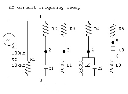 Some of the output from ac.out showing magnitude of
signal at nodes 2, 3, 4, 5 with frequency from
100Hz to 10kHz, note where frequency matches
the parallel tuned circuit at node 4,
and the series tuned circuit at node 5,
at 1kHz.
Note node 2, the capacitor C1 has low impedance at high frequency.
Note node 3. the inductor L1 has high impedance at high frequency.
Circuit: ac.cir ac tuned circuit ngspice -b ac.cir > ac.out
selected output from ac.out
Legend: + = v(2) * = v(3) X = multiple nodes
= = v(4) $ = v(5)
--------------------------------------------------------------------------
frequency v(2) 0.00e+00 2.00e-01 4.00e-01 6.00e-01 8.00e-01 1.00e+00
----------------------|---------|---------|---------|---------|---------|
1.000e+02 9.901e-01 X . . . . X.
1.122e+02 9.876e-01 X . . . . X.
1.259e+02 9.844e-01 X . . . . X.
1.413e+02 9.804e-01 *= . . . . $+.
1.585e+02 9.755e-01 .X . . . . X .
1.778e+02 9.693e-01 .X . . . . X .
1.995e+02 9.617e-01 .*= . . . . $+ .
2.239e+02 9.523e-01 . X . . . . X .
2.512e+02 9.406e-01 . *= . . . . $+ .
2.818e+02 9.264e-01 . *= . . . . $+ .
3.162e+02 9.091e-01 . *= . . . . $+ .
3.548e+02 8.882e-01 . * = . . . . $ + .
3.981e+02 8.632e-01 . * =. . . $ + .
4.467e+02 8.337e-01 . * .= . . $ .+ .
5.012e+02 7.992e-01 . * = . . $ +. .
5.623e+02 7.597e-01 . . * = $. + . .
6.310e+02 7.153e-01 . . * . $ = . + . .
7.079e+02 6.661e-01 . . X . . X . .
7.943e+02 6.131e-01 . $ . *. + .= .
8.913e+02 5.573e-01 . $ . . * + . . = .
1.000e+03 5.000e-01 $ . . X . . =.
1.122e+03 4.427e-01 . $ . . + * . . = .
1.259e+03 3.869e-01 . $ . +. * .= .
1.413e+03 3.339e-01 . . X . . X . .
1.585e+03 2.847e-01 . . + . $ = . * . .
1.778e+03 2.403e-01 . . + = $. * . .
1.995e+03 2.008e-01 . + = . . $ *. .
2.239e+03 1.663e-01 . + .= . . $ .* .
2.512e+03 1.368e-01 . + =. . . $ * .
2.818e+03 1.118e-01 . + = . . . . $ * .
3.162e+03 9.091e-02 . += . . . . $* .
3.548e+03 7.359e-02 . += . . . . $* .
3.981e+03 5.935e-02 . += . . . . $* .
4.467e+03 4.773e-02 . X . . . . X .
5.012e+03 3.829e-02 .+= . . . . $* .
5.623e+03 3.065e-02 .X . . . . X .
6.310e+03 2.450e-02 .X . . . . X .
7.079e+03 1.956e-02 += . . . . $*.
7.943e+03 1.560e-02 X . . . . X.
8.913e+03 1.243e-02 X . . . . X.
1.000e+04 9.901e-03 X . . . . X.
----------------------|---------|---------|---------|---------|---------|
frequency v(2) 0.00e+00 2.00e-01 4.00e-01 6.00e-01 8.00e-01 1.00e+00
Then, nodes 2, 3, 4, 5 plotted on linear frequency scale
Some of the output from ac.out showing magnitude of
signal at nodes 2, 3, 4, 5 with frequency from
100Hz to 10kHz, note where frequency matches
the parallel tuned circuit at node 4,
and the series tuned circuit at node 5,
at 1kHz.
Note node 2, the capacitor C1 has low impedance at high frequency.
Note node 3. the inductor L1 has high impedance at high frequency.
Circuit: ac.cir ac tuned circuit ngspice -b ac.cir > ac.out
selected output from ac.out
Legend: + = v(2) * = v(3) X = multiple nodes
= = v(4) $ = v(5)
--------------------------------------------------------------------------
frequency v(2) 0.00e+00 2.00e-01 4.00e-01 6.00e-01 8.00e-01 1.00e+00
----------------------|---------|---------|---------|---------|---------|
1.000e+02 9.901e-01 X . . . . X.
1.122e+02 9.876e-01 X . . . . X.
1.259e+02 9.844e-01 X . . . . X.
1.413e+02 9.804e-01 *= . . . . $+.
1.585e+02 9.755e-01 .X . . . . X .
1.778e+02 9.693e-01 .X . . . . X .
1.995e+02 9.617e-01 .*= . . . . $+ .
2.239e+02 9.523e-01 . X . . . . X .
2.512e+02 9.406e-01 . *= . . . . $+ .
2.818e+02 9.264e-01 . *= . . . . $+ .
3.162e+02 9.091e-01 . *= . . . . $+ .
3.548e+02 8.882e-01 . * = . . . . $ + .
3.981e+02 8.632e-01 . * =. . . $ + .
4.467e+02 8.337e-01 . * .= . . $ .+ .
5.012e+02 7.992e-01 . * = . . $ +. .
5.623e+02 7.597e-01 . . * = $. + . .
6.310e+02 7.153e-01 . . * . $ = . + . .
7.079e+02 6.661e-01 . . X . . X . .
7.943e+02 6.131e-01 . $ . *. + .= .
8.913e+02 5.573e-01 . $ . . * + . . = .
1.000e+03 5.000e-01 $ . . X . . =.
1.122e+03 4.427e-01 . $ . . + * . . = .
1.259e+03 3.869e-01 . $ . +. * .= .
1.413e+03 3.339e-01 . . X . . X . .
1.585e+03 2.847e-01 . . + . $ = . * . .
1.778e+03 2.403e-01 . . + = $. * . .
1.995e+03 2.008e-01 . + = . . $ *. .
2.239e+03 1.663e-01 . + .= . . $ .* .
2.512e+03 1.368e-01 . + =. . . $ * .
2.818e+03 1.118e-01 . + = . . . . $ * .
3.162e+03 9.091e-02 . += . . . . $* .
3.548e+03 7.359e-02 . += . . . . $* .
3.981e+03 5.935e-02 . += . . . . $* .
4.467e+03 4.773e-02 . X . . . . X .
5.012e+03 3.829e-02 .+= . . . . $* .
5.623e+03 3.065e-02 .X . . . . X .
6.310e+03 2.450e-02 .X . . . . X .
7.079e+03 1.956e-02 += . . . . $*.
7.943e+03 1.560e-02 X . . . . X.
8.913e+03 1.243e-02 X . . . . X.
1.000e+04 9.901e-03 X . . . . X.
----------------------|---------|---------|---------|---------|---------|
frequency v(2) 0.00e+00 2.00e-01 4.00e-01 6.00e-01 8.00e-01 1.00e+00
Then, nodes 2, 3, 4, 5 plotted on linear frequency scale
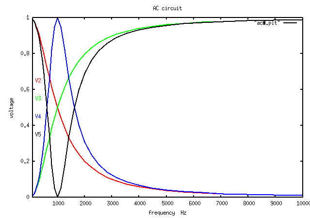
Airfoil lift and drag coefficients
The shape of a moving object determines its drag coefficient, Cd.
The drag coefficient combined with velocity and area of the
moving object determine the drag force.
Fd = 1/2 * Cd * density * area * velocity^2
A few shapes and their respective drag coefficients are:
A symmetric NACA 0015 airfoil at zero degrees angle of attack
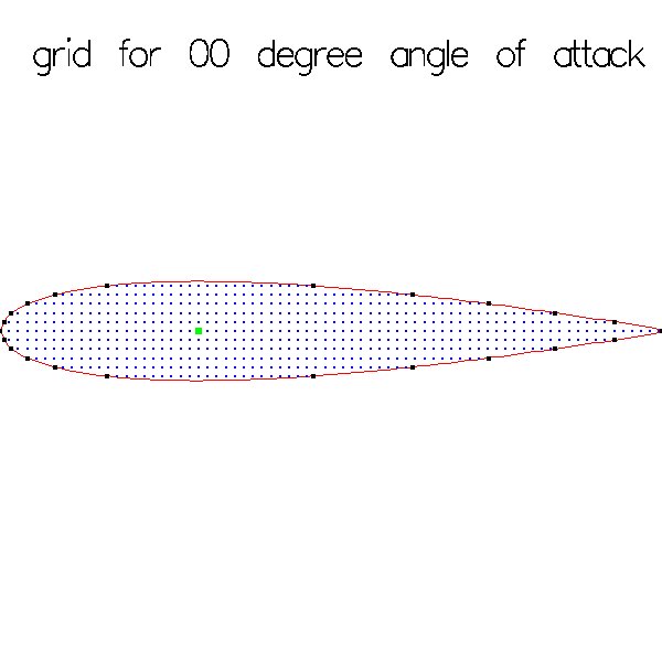 A symmetric NACA 0015 airfoil at 22 degrees angle of attack
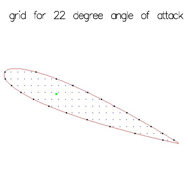 Angle of attack shown in two degree increments
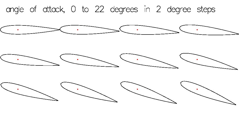 Wind tunnel measured data coefficient of lift and drag
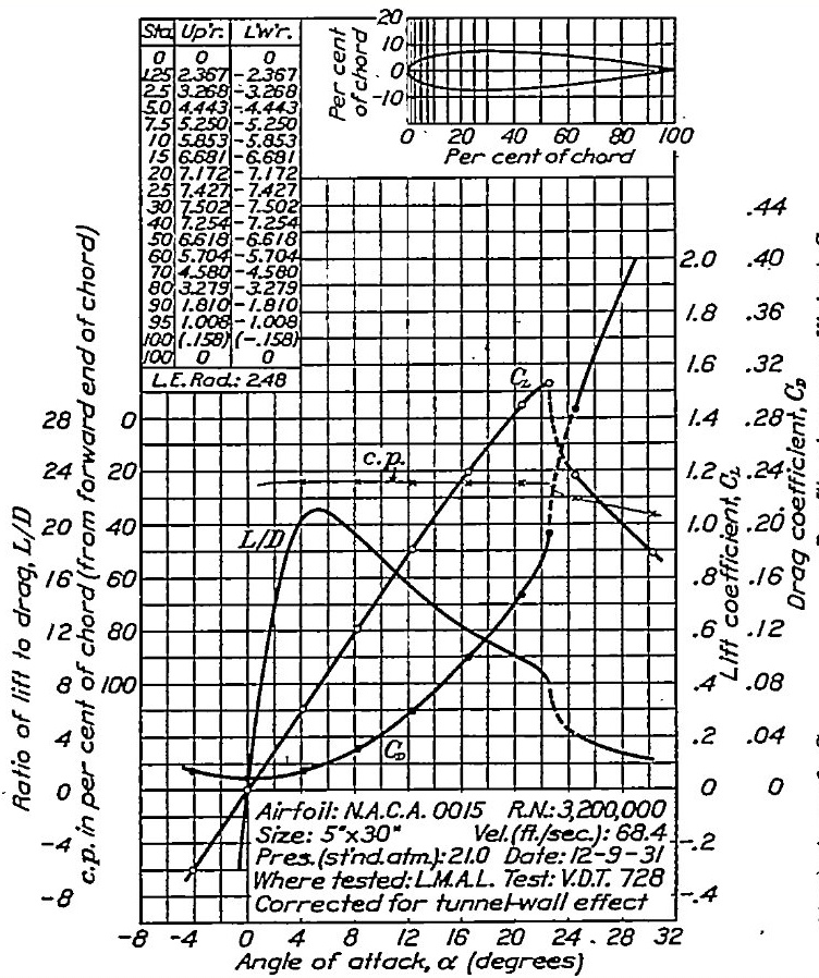 Full set of wind tunnel data and full report
NACA-460 1933 78 airfoils
Source code for computations and plots of airfoils
0015gl.c
0015grid.c
0015grid.out
Observe aircraft from past still flying:
video
Full set of wind tunnel data and full report
NACA-460 1933 78 airfoils
Source code for computations and plots of airfoils
0015gl.c
0015grid.c
0015grid.out
Observe aircraft from past still flying:
video
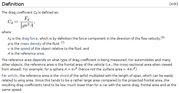 More airflow over cylinder at high Reynolds number:
inertial force ρ u L u L
RE = -------------- = --------- = ------
viscous force μ ν
L is length m = characteristic length, chord for wing, diameter for circle
u is velocity m/s
ρ is density kg/m^3 water 1000 kg/m^3 air 1.275 kg/m^3
μ is dynamic viscosity kg/ms water 0.001 kg/ms air 2*10-5 kg/ms
ν is kinematic viscosity m^2/s water 10^-6 m^2/s air 1.9*10-5 m^2/s
density and viscosity change with temperature, pressure, fluid
Typical flow goes from laminar to turbulent as RE increases above 10
see flow result plots
temperature.shtml degree conversions
work in progress still bugs:
cylinder_flow.c
cylinder_flow_c.out
cylinder_flow.java
cylinder_flow_java.out
More airflow over cylinder at high Reynolds number:
inertial force ρ u L u L
RE = -------------- = --------- = ------
viscous force μ ν
L is length m = characteristic length, chord for wing, diameter for circle
u is velocity m/s
ρ is density kg/m^3 water 1000 kg/m^3 air 1.275 kg/m^3
μ is dynamic viscosity kg/ms water 0.001 kg/ms air 2*10-5 kg/ms
ν is kinematic viscosity m^2/s water 10^-6 m^2/s air 1.9*10-5 m^2/s
density and viscosity change with temperature, pressure, fluid
Typical flow goes from laminar to turbulent as RE increases above 10
see flow result plots
temperature.shtml degree conversions
work in progress still bugs:
cylinder_flow.c
cylinder_flow_c.out
cylinder_flow.java
cylinder_flow_java.out
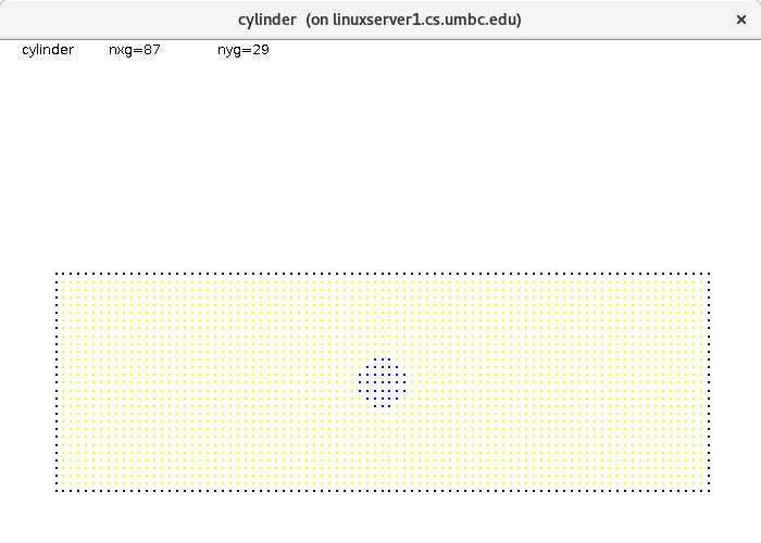 wing_flow.java
wing_flow_java.out
wing_flow.java
wing_flow_java.out
Continuum Hypothesis
The "Continuum Hypothesis" states that the cardinality
of the set of real numbers is two to the power of the
cardinality of the set of integers.
The cardinal number for a set is the size of the set.
There are infinitely many integers, denoted by Ω omega,
or more modern א zero Aleph-Naught.
There are infinitely many reals, denoted by
2^א zero = א one Aleph-One.
The following is called a "proof by picture" that is typically
not accepted by strict mathematicians, yet, this is about
numerical computation.
We will write the real numbers from zero to about one,
as binary fractions. This is a subset of the real numbers
because each fraction may have every integer as its
integer part. We do not even bother to count that when
determining the cardinality of the real numbers.
We use a one-to-many mapping from the integers
to the real fractions. The integer is at the top and
the real fraction runs vertically as binary.
At each step we take each real and make two reals by
appending a zero and one. The number of bits in the
fraction is the mapping from the integer.
Step 1: integer 1 there are 21 reals with 1 fractional bit
real 0.0
0.1
Step 2: integer 2 there are 22 reals with 2 fractional bits
real 0.00
0.01
0.10
0.11
Step 3: integer 3 there are 23 reals with 3 fractional bits
real 0.000
0.001
0.010
0.011
0.100
0.101
0.110
0.111
Step 4: integer 4 there are 24 reals with 4 fractional bits
real 0.0000
0.0001
0.0010
0.0011
0.0100
0.0101
0.0110
0.0111
0.1000
0.1001
0.1010
0.1011
0.1100
0.1101
0.1110
0.1111
The steps continue for all of the integers.
Thus: there are 2n real fractions in the range zero to one
for n integers.
Thus: there are two to the power Omega real fractions.
With a little hand waving, proving by picture that:
There are 2Ω real numbers, א Aleph Null, the cardinality of
the real numbers.
The hand waving is that n 2n becomes 2n as
n becomes infinity.
qed.
Function programming is different
some information on Functional Programming
openMP parallel computation
Reasonably easy way to speed up your program on a computer
with multiple cores. That is almost every computer built
today. Often you can have twice as many threads running
as you have physical cores.
OMP short of openMP is not technically a language.
Pragmas are used in a conventional language to cause the
compiler to generate calls to run time library routines.
Typically, OMP causes tasks to be generated and executed.
Often the underlying task are provided by pthreads.
Fortran and C family compilers usually support OMP.
Some other languages may also provide support.
Specifically with gcc there must be a -fopenmp option
in order for the compiler to process the pragmas.
Each pragma has the syntax #pragma omp ...
With no braces { } the pragma applies to the next statement.
#pragma omp parallel
{
// many copies will be executed
}
test1.c is a first OMP program to run to find out if OMP is
installed and how many tasks are available:
test1.c first test
test1_c.out output from one computer
// test1.c check if openMP available compile gcc -fopenmp ...
#include
#include
#include
#include
int main(int argc, char * argv[])
{
int myid;
int def_num_threads, num_threads, num_proc;
double ttime;
num_proc = omp_get_num_procs();
printf("test1.c check for openMP, num_proc=%d \n", num_proc);
fflush(stdout);
ttime = omp_get_wtime(); // wall time now, in seconds
#pragma omp parallel // must be at least one "parallel", else no threads
{
#pragma omp master // only the master thread will run { to }
{
def_num_threads = omp_get_num_threads(); // must be in parallel
omp_set_num_threads(6);
num_threads = omp_get_num_threads();
printf("def_num_threads=%d, try 6, omp_set_num_threads =%d \n",
def_num_threads, num_threads);
fflush(stdout); // needed to get clean output
}
#pragma omp barrier // all threads must be doing nothing
myid = omp_get_thread_num(); // master == 0
printf("test1.c in pragma omp parallel myid=%d \n", myid);
fflush(stdout);
}
// total wall time is difference
printf("test1.c ends, %f seconds \n", omp_get_wtime()-ttime);
fflush(stdout);
return 0;
} // end test1.c
On one of my computers the output is:
test1.c check for openMP, num_proc=8
def_num_threads=8, try 6, omp_set_num_threads =8
test1.c in pragma omp parallel myid=0
test1.c in pragma omp parallel myid=1
test1.c in pragma omp parallel myid=4
test1.c in pragma omp parallel myid=7
test1.c in pragma omp parallel myid=6
test1.c in pragma omp parallel myid=5
test1.c in pragma omp parallel myid=2
test1.c in pragma omp parallel myid=3
test1.c ends, 0.039330 seconds
As you can see, my system would not do the
omp_set_num_threads(6); it used the default.
The fflush(stdout); is used after every printf, else
output lines from various threads may get intertwined.
There is an on-line tutorial for openMP by an Intel developer.
This tutorial takes a few hours and has programming assignments.
https://www.youtube.com/watch?v=nE-xN4Bf8XI
One of the problems is to take a sequential program with a
loop and parallelize the program. The program does numerical
integration to compute the value of Pi. 3.14159...
The next sequence of files, you need to click to see them,
is a more extensive version of the tutorial problem.
First the non parallel program, I always check my code before parallelizing:
pi.c a non parallel version for test and timing
pi_c.out output of non parallel version
pi.make Makefile for single computer
Source code with OMP pragmas, source, output, Makefile
pi_omp.c source code with openMP pragmas
pi_omp.out output, many more cases, parallel
pi_omp.make OMP Makefile for single computer
Same source code run on a cluster, uses slurm and activated by mpi
pi_omp.slurm driver code only for cluster
pi_omp.makeslurm Makefile for cluster
Some key points:
#pragma omp parallel // if declared above, could say private(x)
{
double x; // a different location for each thread
#pragma omp for reduction(+:pi) says each task will be adding to pi,
avoid race condition on update,
much faster than #pragma omp atomic yet does same thing.
Now, what if you have nested loops that are smaller than
number of available threads, tasks?
test2.c parallelize nested loops
test2_c.out output showing which thread is running
Here, "static" option, rather than "dynamic" option was used because
all threads take about the same time.
Notice that the use of threads, myid, is not equal.
Functional Programming and Functional Languages
Functional Programming and Functional Languages
From Wikipedia:
In computer science, functional programming is a programming paradigm,
a style of building the structure and elements of computer programs,
that treats computation as the evaluation of mathematical functions
and avoids state and mutable data. Functional programming emphasizes
functions that produce results that depend only on their inputs and
not on the program state.i.e. pure mathematical functions.
It is a declarative programming paradigm, which means programming
is done with expressions. In functional code, the output value of
a function depends only on the arguments that are input to the function,
so calling a function f twice with the same value for an argument x
will produce the same result f(x) both times. Eliminating side effects,
i.e. changes in state that do not depend on the function inputs,
can make it much easier to understand and predict the behavior
of a program, which is one of the key motivations for the development
of functional programming.
Functional programming has its roots in lambda calculus,
a formal system developed in the 1930s to investigate computability,
the Entscheidungsproblem, function definition, function application,
and recursion. Many functional programming languages can be viewed
as elaborations on the lambda calculus, where computation is treated
as the evaluation of mathematical functions and avoids state and
mutable data. In the other well known declarative programming paradigm,
logic programming, relations are at the base of respective languages.
In contrast, imperative programming changes state with commands
in the source language, the most simple example is the assignment.
Functions do exist, not in the mathematical sense, but in the sense
of subroutine. They can have side effects that may change the value
of program state. Functions without return value therefore make sense.
Because of this, they lack referential transparency,
i.e. the same language expression can result in different values
at different times depending on the state of the executing program.
Functional programming languages, especially purely functional ones
such as Hope and Rex, have largely been emphasized in academia
rather than in commercial software development. However, prominent
functional programming languages such as Common Lisp, Scheme, Clojure,
Racket, Erlang, OCaml, Haskell, and F# have been used in industrial
and commercial applications by a wide variety of organizations.
Functional programming is also supported in some domain-specific
programming languages like R (statistics), Mathematica
(symbolic and numeric math), J, K and Q from Kx Systems (financial analysis),
XQuery/XSLT (XML), and Opal. Widespread domain-specific declarative
languages like SQL and Lex/Yacc use some elements of functional programming,
especially in eschewing mutable values.
Programming in a functional style can also be accomplished in languages
that aren't specifically designed for functional programming.
For example, the imperative Perl programming language has been the
subject of a book describing how to apply functional programming concepts.
C# 3.0 and Java 8 added constructs to facilitate the functional style.
An interesting case is that of Scala - it is frequently written in
a functional style, but the presence of side effects and mutable state
place it in a grey area between imperative and functional languages.
SML example
gauss.sml solve simultaneous equations
gauss.out output
See Wikipedia for references.
wiki functional programming
CMSC 455 Numerical Computation lectures
Other links
-
CMSC 455 home page
-
Syllabus - class dates and subjects, homework dates, reading assignments
-
Homework assignments - the details
-
Projects -
-
Partial Lecture Notes, one per WEB page
-
Partial Lecture Notes, one big page for printing
-
Downloadable samples, source and executables
-
Some brief notes on Matlab
-
Some brief notes on Python
-
Some brief notes on Fortran 95
-
Some brief notes on Ada 95
-
An Ada math library (gnatmath95)
-
Finite difference approximations for derivatives
-
MATLAB examples, some ODE, some PDE
-
parallel threads examples
-
Reference pages on Taylor series, identities,
coordinate systems, differential operators
-
selected news related to numerical computation
Go to top
Last updated 10/23/2014
