Basic operations in Excel

The basic operations that you need to know how to do in Excel are the following:

    1.  Entering numbers into cells

    2.  Entering text into cells

    3.  Entering formulas into cells

    4.  Editing cells containing numbers, text, or formulas.

    5.  Use of functions (such as exp, ln, sum, ave, etc.)

    6.  Specifying ranges of cells for use in functions

    7.  Use of the copy command for formulas, including the effect of using relative and absolute addresses when copying cells.

    8.  Setting the recalculation options (using <tools\options\calculation>) to manual or automatic.

    9.  Use of the solver feature.

Financial Functions

A number of financial functions are also available in Excel that are sometimes useful, such as the internal rate of return, IRR(*), where * is a range specifying the cash flow.  For example, the rate of return for a $10,000 investment in year 1 which returns $3,000 in year 2, $3,000 in year 3,  $4,000 in year 4, and $4,000 in year 5 can be determined by entering the values -10000, +3000, +3000, +4000, and +4000 in cells A1 to A5 and then evaluating =IRR(A1:A5) entered in another cell.   The result is 14%, indicating a 14% per year return on the original $10,000 investment.

Solution of Nonlinear Constrained Optimization Problems

The solution of a system of nonlinear algebraic equations, or the solution of a nonlinear constrained optimzation problem, can be performed in Excel using the solver feature, which may need to be installed as an add-in. In Excel 2010 (or later) this can be done by using the file/options/add-in menu in Excel. The solver dialog box is shown below and is used to specify the problem. Note that in Excel 2010 (or later) the solver feature is located in the data menu after it is installed, as also shown below.  

As an illustrative example, consider the following constrained optmization problem:  

    Minimize: exp(-x)*(x - 3)^2 + exp(-y)*(y - 2)^2  

    Subject to -x + y ≤ 0 and x + y ≤ 1 where x > 0 and y >0  

As illustrated in the graph below, in this problem it is desired to find the minimum value of exp(-x)*(x-3)^2 + exp(-y)*(y-2)^2 in the yellow triangular region shown. The global minimum of exp(-x)*(x-3)^2 + exp(-y)*(y-2)^2 is zero since this expression is the sum of two terms, both of which must be greater than or equal to zero, and where the first term depends solely on x and the seond term depends solely on y. Also, for finite x and y, this global minimum occurs at the point (x,y) = (3,2) where each of the two terms are individually zero. The global minimum point is also shown in the figure below.  

After installing the solver feature, the problem described above can be setup as shown below. Note that the cells containing the values of x and y shown below have been set at their starting guess values. The solver will change these values to solve the problem when the solve button is pushed in the solver dialog box  

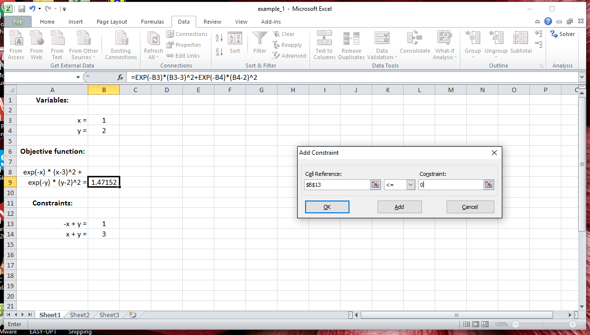
To solve this constrained optimization problem, specify the independent variables for the problem in the Excel spreadsheet as the variable cells to be changed in the solver dialog box. Then specify in the solver dialog box that the cell containing the objective function is to be minimized. The constraints can then be specified using the constraints dialog box shown below.

The options button on the solver dialog box sets the options using the options dialog box as shown below.

The most important options to set are the following:

Solving Method?: GRG Nonlinear (This option selects the generalized reduced gradient method which works well for most problems especially if, for very nonlinear problems, you also select the random multistart option with ~1000 restarts. This makes the solver search for the solution using the specified number of random starting guesses in addition to the specific starting guess that you provide by your initial selection of values in the cells containing the variable cells. The other option for a solution method in the Excel solver feature is the evolutionary genetic algorithm.)

Use automatic scaling?:  yes  (This feature significantly helps in general to achieve convergence, and is essential to use when some independent variables have much larger values than others)

Maximum time:  200 s    (This is the maximum time the solver will run to achieve a solution)

Maximum iterations:  500  (This is the maximum number of interations the solver will perform).

Precision:    0.00001   (This controls how precise equality contraints are satisfied)

Covergence:  0.00001   (This controls how precisely the target  is minimized or maximized.

Solving Systems of Nonlinear Equations

For the case where a system of nonlinear algebraic equations is to be solved but where there is no objective function to optimize, you can leave the objective function cell location blank. For convenience, write the equations to be solved in residual form where the right hand side is zero and the left hand side is the residual expression. Then use the solver dialog box to specify that the locations of the independent variables in the spreadsheet are the variable cells to be changed by the solver. Next, enter the formulas for the residual expressions for each equation to be solved in the spreadsheet such that these residual expressions refer to the locations of the variable cells as appropriate. The cells containing the residual expressions should be zero at the solution, so these cells can be used within equality constraints in the solver dialog box such that they are forced to be zero by having the solver change the variable cells. Finally, you can assist the solver to find the solution by enforcing any known constraints on the independent variable cells, such as constraining an independent variable cell to be within certain limits.

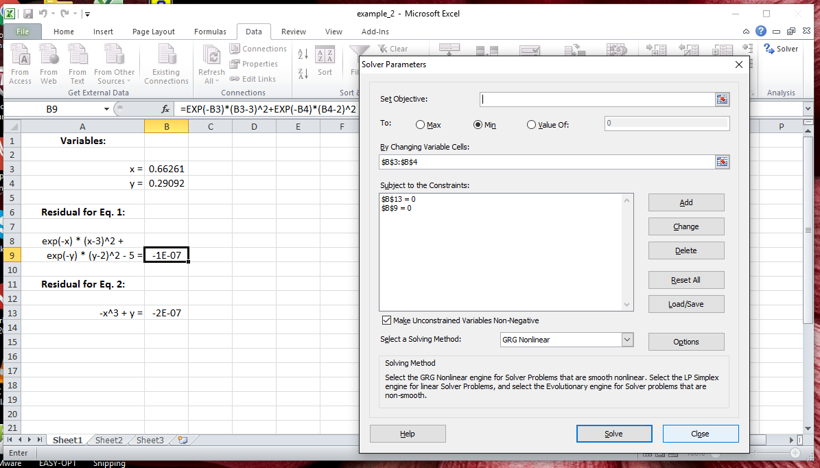
Consider as an example the problem of solving the following two equations:

    exp(-x)*(x-3)^2 + exp(-y)*(y-2)^2 - 5 = 0

    y - x^3 = 0

The spreadsheet shown below illustrates the simultaneous solution of the above two equations using the strategy just described.

Enhancements and Alternatives to the Native Solver in Excel

The solver used in Microsoft Excel was created by the company Frontline Systems. Several upgrades for the existing solver in Excel which enhance it's abilities, some of which are free, are available from this company. Another option for enhancing the abilities of the solver in Excel is to use the free alterntive solver add-in for Excel that is available at the opensolver.org website. The relevant links are given below.

Solving Systems of Ordinary Differential Equations

Excel can also be used to solve a set on nonlinear ordinary differential equations by using, e.g., Euler's method, and then setting up a grid of the independent variable and the values of the dependent variables.  The copy command is used to minimize the amount of effort required to enter formulas. More details can be found in the links given below. 

MATLAB and POLYMATH

Other options for solving algebraic or differential equations numerically are to use MATLAB (or Octave) or POLYMATH. Details are described in the links shown below.

• Frontline Systems. This company created the solver in Excel. They also provide a number of upgrades to the Excel solver add-in, some of which are free and some of which you need to pay for.

 

• OpenSolver for Excel. This website provides alternative solver add-ins for Excel that are available for free. One option that is available for very large and very nonlinear problems is to use Excel as a front end interface for running problems for free on the NEOS (Network Enabled Optimization System) high-performance computing facility located at the University of Wisconsin. If OpenSolver does not load after you upzip the downloaded files, you may need to upblock the zipped files before you unzip them. The instructions for doing this are located here. Additional troubleshooting help is located here. After you unzip the OpenSolver downloaded files and open the OpenSolver.xlma file that is created (where the extension xlma denotes an Excel macro enabled add-in file), OpenSolver will be available until you close Excel. To avoid the need for a fresh "unzipping" whever you want to use OpenSolver, select a subfolder in your Documents folder (or any folder other than your Downloads folder) as the destination when you unzip the downloaded files. You can also then create a Desktop shortcut for the OpenSolver.xlam file in this subfolder. A basic tutorial on using OpenSolver is located here.

 

• Octave. An open-source free MATLAB clone originally developed at the University of Wisconsin.

 

• Using Excel to solve systems of ODEs. This link is from the Mr. Idea Hamster website which, despite its humorous name, contains lots of useful information.