Project 7
A finite elements solver for the Poisson problem in 2D
with zero Dirichlet boundary conditions

To simplify your work, I suggest the following change relative to the textbook.

• Break up the monolithic problem-spec.c into individual problem specification files
  • square-spec.c
  • annulus-spec.c
  • triangle-with-hole-spec.c
  • three-holes-spec.c
  for the four domains, but keep problem-spec.h intact because it is domain-independent and defines the structures that are needed in *-spec.c files.

  This project focuses on the square and annulus domains for which we have exact solutions. Do the other two domains also if you wish, but that's optional.

  Make a header file for each *-spec.c file. Here is the complete annulus-spec.h:

  #ifndef H_ANNULUS_SPEC_H
  #define H_ANNULUS_SPEC_H
  
  #include "problem-spec.h"
  
  struct problem_spec *get_spec_annulus(int n);
  void free_annulus(struct problem_spec *spec);
  
  #endif // H_ANNULUS_SPEC_H
  

• Solve the Poisson problem $\Delta u + f = 0$ on the various domains. I suggest the following choices of $f$.
  1. On the $(0,1)\times(0,1)$ square take $f(x,y) = 32 \bigl(x(1-x) + y(1-y)\bigr)$. This corresponds to the exact solution $u(x,y) = 16x(1-x)y(1-y)$ which you may use to ascertain the solver's accuracy. Thus, in square-spec.c define

     static double f(double x, double y)
     {
     	return 32*(x*(1-x) + y*(1-y));
     }
     
     static double exact(double x, double y)
     {
     	return 16*x*y*(1-x)*(1-y);
     }
     

     and then insert f() and exact() in the problem_spec structure:

     static struct problem_spec spec = {
     	.points         = points,
     	.segments       = segments,
     	.holes          = NULL,
     	.npoints        = (sizeof points)/(sizeof points[0]),
     	.nsegments      = (sizeof segments)/(sizeof segments[0]),
     	.nholes         = 0,
     	.f              = f,		// here it is!
     	.g              = NULL,
     	.h              = NULL,
     	.eta            = NULL,
     	.u_exact        = exact,	// here it is!
     };
     

     Here is what I get:

      ./demo-square 5 0.01
     domain is a square
     nodes = 96, edges = 254, elems = 159
     system stiffness matrix is 96x96 (=9216) has 424 nonzero entries
     errors: L^infty = 0.0413703, L^2 = 0.0154083, energy norm = 0.388679
     pyplot output written to file demo-square.py
     

     Verify that the $L^2$ error is proportional to $a$ (the maximal triangle area) as $a$ approaches zero.

  2. On the annulus, take $\ds f(x,y) = \frac{s}{r^2} \Bigl[ 8 (a+b) r - 9 a b - 5 r^2 \Bigr] \cos3t$, where $a$ and $b$ are the inner and outer radii, and $s = 2/(b-a)$.

     Here $f$ is defined in terms of the polar coordinates $r$ and $t$. We have $r = \sqrt{x^2+y^2}$ and $t = \tan^{-1}(y/x)$. Use the C Standard Library's atan2 for the inverse tangent, as in t = tan2(y,x).

     The exact solution in this case is $u=s(r-a)(b-r) \cos 3t$. Use that to determine the accuracy of the solver.

     Due to poor design, our function $f$ does not take optional arguments as parameters. (Refer to the Nelder-Mead project to see how optional parameters are handled.) For now, you may set the parameters $a$, $b$, and $s$ as preprocessor macros in annuluc-spec.c, as in

     #define a       0.325
     #define b       (2*a)
     #define s       2.0/(b-a)
     

     That works, but such abuse of preprocessor macros is considered poor style. If you feel motivated, see if you can change things to allow parameters in each of the functions f, g, h, η, u_exact that are declared in problem-spec.h. For instance, you may want to change the line

     double (*f)(double x, double y);
     

     to

     double (*f)(double x, double y, void *params);
     

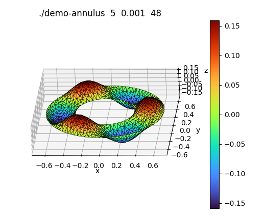
     to allow passing parameters to f.

     Here is what I get:

     ./demo-annulus 5 0.001 48
     domain is an annulus (really a 48-gon) of radii 0.325 and 0.65
     nodes = 860, edges = 2436, elems = 1576
     system stiffness matrix is 860x860 (=739600) has 4830 nonzero entries
     errors: L^infty = 0.00554751, L^2 = 0.00199565, energy norm = 0.146381
     pyplot output written to file demo-annulus.py
     

  3. [Optional] On triangle-with-hole take $f(x,y) = 30 x y (2-x) (2-y)$.

  4. [Optional] On three-holes take $f(x,y) = 15.0$.

• Write program files plot-with-python.c and plot-with-python.h that provide a function plot_with_python() which receives the solution of your FEM solver and writes a python script for plotting the solution's 3D graph. Here is my plot-with-python.h:

  #ifndef H_PLOT_WITH_PYTHON_H
  #define H_PLOT_WITH_PYTHON_H
  
  #include "mesh.h"
  
  void plot_with_python(struct mesh *mesh, char **argv, char *filename);
  
  #endif // H_PLOT_WITH_PYTHON_H
  

  The purpose of passing argv to that function is so that it can put the command-line arguments in the graph's title (see below). The filename argument is the name of the output file.

  Here is an sample python script that plots a surface consisting of two triangles.

  # --- A --------------------------------#
  import numpy as np
  import matplotlib.pyplot as plt
  from mpl_toolkits.mplot3d import Axes3D
  from matplotlib import cm
  fig = plt.figure()
  ax = fig.add_subplot(111, projection='3d')
  ax.set_proj_type('ortho')
  
  # --- B --------------------------------#
  ax.set_title('Your Title Here')	// optional: set title 
  
  coords = np.array([
  	[0, 0, 0],
  	[1, 0, 0],
  	[1, 1, 1],
  	[0, 1, 0.5],
  ])
  
  elems = np.array([
  	[0, 1, 2],
  	[0, 2, 3],
  ])
  
  # --- C --------------------------------#
  x = coords[:, 0]
  y = coords[:, 1]
  z = coords[:, 2]
  surf = ax.plot_trisurf(x, y, z, triangles=elems,
  	cmap=cm.turbo, edgecolor='black', linewidth=0.4)
  fig.colorbar(surf, shrink=0.75)
  ax.set_xlabel('x')
  ax.set_ylabel('y')
  ax.set_zlabel('z')
  ax.set_aspect('equal') # requires matplotlib version >= 3.6
  plt.show()
  # --------------------------------------#
  

  The group of lines marked A and C are independent of the particular problem. Only those in group B vary. The array coords consists of the coordinates $[x_i, y_i, z_i]$, $i=0,1,2,\ldots$ of the surface's points. The array elems consists of the indices $[v^{(i)}_0, v^{(i)}_1, v^{(i)}_2]$, $i=0,1,2,\dots$ of element vertices.

  Optionally, you may set the plot's title through the set_title line shown above. I like to set it to command-line arguments which are available through the argv array in main(). Here is a sample: