If you are running R, connected to the internet, and have write privileges on your computer's disk, you can
install GrassmannOptim by typing the following command in the R command window:
> install.packages("GrassmannOptim")
To use the GrassmannOptim package you must enter the library command in R:
> library(GrassmannOptim)
Some Optimization Examples Using GrassmannOptim
The following are some examples of the use of GrassmannOptim package.
Example 1:
Likelihood Acquired Direction (Cook and Forzani, 2009).
Is it a car, a plane, a bird? The package is used to reproduce the result of Cook and Forzani (2009). Figure 1 shows the plot of the two direstions obtained from the optimization.
The dataset is can be accessed here.
lad = function(X, y, d=1,...)
{
	# The following code assume that
	# X is a n x p data-matrix and y is a
	#Initialization
	mf <- match.call()
	op <- dim(X);
	p <- op[2]
	n <- op[1]
	if (p > n) stop("This method requires n larger than p")
	Xc <- scale(X, TRUE , FALSE)
	Sigmatilde <- t(Xc)%*%Xc/n

	projection <- function(alpha, Sigma)
	{	return(alpha%*%solve(t(alpha)%*%Sigma%*%alpha)%*%t(alpha)%*%Sigma)
	}

	groups <- unique(sort(y))
	nSlices <- length(groups)
	N_y <-vector(length=nSlices)
	Deltatilde_y = vector(length=nSlices, "list")
	for (i in 1:nSlices)
	{	N_y[i] <- length(y[y==groups[i]])
		X_y <- X[which(y == groups[i]),]
		X_yc <- scale(X_y, TRUE, FALSE)
		Deltatilde_y[[i]] <- t(X_yc)%*%(X_yc)/N_y[i]
	}
	Sigmas <- list(Sigmatilde=Sigmatilde, Deltatilde_y=Deltatilde_y, N_y=N_y)
  	Deltatilde <- 0
	for (i in 1:nSlices) Deltatilde <- Deltatilde + N_y[i]*Deltatilde_y[[i]]

	if ((d==0)|(d==p)) return("This code is not designed for that dimension")

	if ((d!=0)&(d!=p))
	{
		objfun <- function(W)
		{
			Q <- W$Qt
			d <- W$dim[1]
			p <- W$dim[2]
			Sigmas <- W$Sigmas
			n <- sum(Sigmas$N_y)
			U <- matrix(Q[,1:d], nc=d)
			V <- matrix(Q[,(d+1):p], nc=(p-d))

			# Objective function
			terme0 <- -(n*p)*(1+log(2*pi))/2
			terme1 <- -n*log(det(Sigmas$Sigmatilde))/2
			term <- det(t(U)%*%Sigmas$Sigmatilde%*%U)
			if (is.null(term)|is.na(term)|(term <= 0)) return(NA) else terme2 <- n*log(term)/2
			terme3<-0
			for (i in 1:length(Sigmas$N_y))
			{
				term <- det( t(U)%*%Sigmas$Deltatilde_y[[i]]%*%U )
				if (is.null(term)|is.na(term)|(term <=0)) {break; return(NA)}
				terme3 <- terme3 - Sigmas$N_y[i]*log(term)/2
			}
			value <- terme0 + terme1 + terme2 + terme3

			#Gradient
			terme0 <- solve(t(U)%*%Sigmas$Sigmatilde%*%U)
			terme1 <- sum(Sigmas$N_y) * t(V)%*%Sigmas$Sigmatilde%*%U%*%terme0
			terme2 <- 0
			for (i in 1:length(Sigmas$N_y))
			{
				temp0 <- solve(t(U)%*%Sigmas$Deltatilde_y[[i]]%*%U)
				temp <-Sigmas$N_y[i]*t(V)%*%Sigmas$Deltatilde_y[[i]]%*%U%*%temp0
				terme2 <- terme2 - temp
			}
			gradient <- t(terme1 + terme2)
			return(list(value=value, gradient=gradient))
		}
		objfun <- assign("objfun", objfun, env=.GlobalEnv)
		W <- list(dim=c(d,p), Sigmas=Sigmas)
		grassmann <- GrassmannOptim(objfun, W,...)
	}
	return(matrix(grassmann$Qt[,1:d], ncol=d))
}

dat <- read.table(url("http://www.math.umbc.edu/~kofi/GrassmannOptim/marcewhole.txt"), header=FALSE)
Gm <- lad(X=dat[,-1], y=dat[,1], d=2, sim_anneal=TRUE, cooling_rate = 1.2, max_iter_sa=200, max_iter=400, verbose=TRUE)
V<- t(Gm)%*%t(dat[,-1])

mycol <- dat[,1]
mycol[mycol==0]<-"black"
mycol[mycol==1]<-"blue"
mycol[mycol==2]<-"green"

jpeg(filename = "carplanebird.jpg")
plot(V[1,], V[2,], xlab="Dir1", ylab="Dir2", pch=as.numeric(dat[,1]), cex=1.50, col=mycol);
title(main="Figure 1")
dev.off();
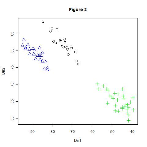
Example 2:
This second example also uses LAD on the flea beetles data (The GGobi book, Dianne Cook and Deborah F. Swayne). Figure 2 is the outpout of the data projected on the
two directions obtained by the Grassmann optimization.
dat <- read.csv(url("http://www.ggobi.org/book/data/flea.csv"), header=TRUE)
Levels <- unique(dat[,1]); y <- length(dat[,1]); X <- dat[,-1]
for (i in 1:length(Levels)) y[dat[,1]==Levels[i]] <- i

Gm <- lad(X=X, y=y, d=2, sim_anneal=TRUE, cooling_rate=1.2, max_iter_sa=200, max_iter=400, verbose=TRUE)
V<- t(Gm)%*%t(X)

mycol <- y
mycol[mycol==1]<-"black"
mycol[mycol==2]<-"blue"
mycol[mycol==3]<-"green"

jpeg(filename = "fleaLAD.jpg")
plot(V[1,], V[2,], xlab="Dir1", ylab="Dir2", pch=as.numeric(y), cex=1.50, col=mycol)
title(main="Figure 2")
dev.off();
Example 3:
I consider using LDA Projection Pursuit index of Lee and Cook (2009) on the flea beetles data. Figure 3 shows the corresponding output.
dat <- read.csv(url("http://www.ggobi.org/book/data/flea.csv"), header=TRUE)
n <- nrow(dat)# The number of observations
Levels <- unique(dat[,1])# The classes or groups
nLevels <- length(Levels) # The number of groups or classes

y <- vector(length=n); X <- dat[,-1]
for (i in 1:nLevels) y[dat[,1]==Levels[i]] <- i; # labeling classes by 1,2,3.
N_y <-vector(length=nLevels);
for (i in 1:nLevels) N_y[i] <- length(y[y==i])
xbar_y = vector(length=nLevels, "list")
xbar <- apply(X, 2, mean)

B <- 0; # Between-group sum of squares
A <-0; # within-group sums of squares
tempX <- vector("list")

for (i in 1:nLevels){
	tempX[[i]] <- X[y==i,]
	B <- B + N_y[i]*(apply(X[y==i,], 2, mean) - xbar)%*%t(apply(X[y==i,], 2, mean) - xbar)
	temp <- 0
	for (j in 1:N_y[i]){
		terme0 <- matrix(as.numeric(tempX[[i]][j,] - apply(tempX[[i]], 2, mean), nc=1))
		temp <- temp + terme0%*%t(terme0)
	}
	A <- A + temp
}
proj_index <- function(W){
	det(t(W$U)%*%W$A%*%W$U)/det(t(W$U)%*%(W$A + W$B)%*%W$U)
}
Qt <- OrthoNorm(matrix(runif(36), ncol=6))
W <- list(dim=c(2, 6), Qt=Qt, U=Qt[,1:2], V=Qt[, 3:6], A=A, B=B)
pp_opt <- function(W) return(list(value=proj_index(W)))

ans <- GrassmannOptim(pp_opt, W, sim_anneal = TRUE, cooling_rate = 1.2, max_iter_sa=200, max_iter=400, verbose = TRUE)

mycol <- y
mycol[mycol==1]<-"black"
mycol[mycol==2]<-"blue"
mycol[mycol==3]<-"green"

jpeg(filename = "fleaLDAPP.jpg")
plot(t(ans$Qt[,1])%*%t(X), t(ans$Qt[,2])%*%t(X), xlab="Dir1", ylab="Dir2", pch=as.numeric(y), cex=1.50, col=mycol)
title(main="Figure 3")
dev.off();
Example 4:
This example uses the usual LDA function f(U)=U'BU(U'AU)^{-1}. A Grassmann optimization is performed to separate the classes on the flea beetles data.
Figure 4 shows its output.
From www.r-project.org, the home for R, you can get a wealth of information about the software R. The help file of GrassmannOptim available from the R Help menu is also useful.
References
Cook RD, Forzani L (2009) Likelihood-based Sufficient Dimension Reduction, J. of the American Statistical Association, Vol. 104, No. 485, 197--208.
Lee E-K, Cook D (2009) A Projection Pursuit Index for Large p Small n Data, Statistics and Computing
The views and opinions expressed in this page are strictly those of the page author.
The contents of this page have not been approved by the University of Maryland.
This page was last modified on December 12, 2011 21:17