Due:Monday, September 29, by noon

Introduction: This problem set is based on material in Chapters 2 and 3. This problem set is designed to familiarize you with locating economic data on the internet and with the time series decomposition of economic variables. The problem set also provides additional experience with the linear regression feature found in spreadsheets and statistical concepts from Chapter 6.

Solution: ps_1_solution.xls (Excel Spreadsheet)

Problem Set Questions:

1. Describe the four data series on the file. What does each measure?
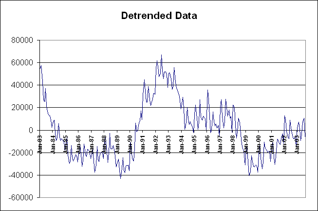
   The series are monthly and run from January 1983 through August 2003. These series measure the conditions of the labor market in Maryland. The individual series are:
   1. labor force: The labor force, or the number of workers available to fill jobs in the economy, comprises all civilians 16 years of age or older who are either working or looking for work. The labor force does not include institutionalized workers, such as prison inmates.
   2. employment: The number of persons in the labor force who have a job.
   3. unemployment: The number of persons in the labor force who are actively looking for a job.
   4. unemployment rate: (unemployed)/(labor force)
2. Graph the unemployment series over the 1983-2003 period.

   

3. Describe the time series properties of this series that you can see on the graph, in the context of the additive time series decomposition
   Y = T+S+C+I
   There is no appearant secular trend in the variable. The number of persons looking for work in Maryland has not grown over the past twenty years. There is a lot of high frequence variation that may be seasonal variation in persons looking for work. There appears to be a cyclical component to the series. The number of unemployed persons fell steadily through the 1980s, a long expansion, rose in the early 1990s, a recession, fell through the mid to late 1990s and then rose again in late 2000. The drop in the number of unemployed in 1999 may be an irregular component, as there was no business cycle downturn in the US at that time.
4. Remove the deterministic trend from the series using an appropriate regression model. Discuss the form of the trend you removed, write down the equation for this model, include the regression results in your spreadsheet, and discuss the results of this regression. Your spreadsheet file should include a seperate sheet with the detrended series clearly labled detrended!
   The secular trend can be removed in many ways. The simplest would be an additive linear trend. An additiative linear trend can be removed using the regression model U_t = a₀ + a₁T_t + e_t
   where T_t is a sequence of integers beginning at one in January 1983 and increasing by one each month. a₀ is the intercept and a₁ the slope parameter, showing by how much unemployment increased each month. e_t is the equation error term capturing all other factors that affect unemployment. Estimating this model gives

   Regression Statistics				
   Multiple R            0.032			
   R Square              0.001			
   Adjusted R Square    -0.003
   Standard Error        24891			
   Observations            248			
   
   ANOVA				
                df          SS      MS             F
   Regression    1   161953859.2   161953859.2    0.261
   Residual    246    1.52422E+11  619603545.8	
   Total       247    1.52584E+11		
   				
                  Coefficients Standard Error t Stat
   Intercept             125432   3170.8        39.55
   X Variable 1         11.2878    22.07         0.51
   

5. Graph the detrended data; label this graph "Detrended Data" and put it in your spreadsheet file. Describe the time series properties of this detrended series.

   

   The parameter on the trend variable in the regression model was not statistically different from zero, confirming the visual inspection above. There is no secular trend in the number of persons unemployed in Maryland over the sample period. Because the trend term is not significant, the detrended series simply removes the mean from the series. All other time series features are still present, the series has been shifted down by 125432 each month.

6. Remove the seasonal variation in the detrended series. Use a 12 month moving average to remove the seasonal factors. Start this moving average in November 1983. Graph both the detrended series and the seasonally adjusted series on the same axes. Label this graph "Seasonally Adjusted data" and include it in your spreadsheet file.

   

7. Discuss the merits and weaknesses of this detrending and seasonal adjustment process. What alternatives could you have used?