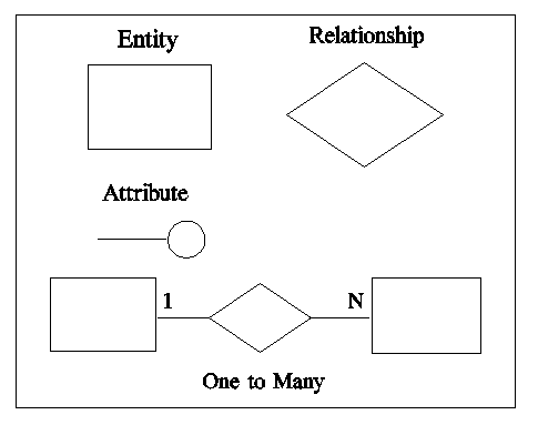
 Figure
C1 - Symbols used in an entity relationship diagram.
Figure
C1 - Symbols used in an entity relationship diagram. by Carol E. Brown, CPA, PhD
Information and data are different. Information is understood by a person. Data are patterns stored on a passive medium like a computer disk. The purpose of a database system is to bridge the gap between information and data - the data stored in memory or on disk must be converted to usable information.
A database is a model of a real world system. The contents (sometimes called the extension) of a database represent the state of what is being modeled. Changes in the database represent events occurring in the environment that change the state of what is being modeled. It is appropriate to structure a database to mirror what it is intended to model.
Databases can be analyzed on different levels:
Conceptual-level - Semantic data models
(High level - not system specific)
Application-level
Conceptual-level concepts permit us to model the application world in terms independent of any particular data model. They are a convenient mechanism to allow the structure of a database to evolve over time as the environment being modeled, user needs and information requirements change. Conceptual models provide a framework for developing a database structure or schema from the top down. One very popular conceptual-level model is the entity-relationship model.
The entity-relationship model is a tool for analyzing the semantic features of an application that are independent of events. This approach includes a graphical notation which depicts entity classes as rectangles, relationships as diamonds, and attributes as circles or ovals. For complex situations a partial entity-relationship diagram may be used to present a summary of the entities and relationships but not include the details of the attributes.
The entity-relationship diagram provides a convenient method for visualizing the interrelationships among entities in a given application. This tool has proven useful in making the transition from an information application description to a formal database schema. The entity-relationship model is used for describing the conceptual scheme of an enterprise without attention to the efficiency of the physical database design.
The entity-relationship diagrams are later turned into a conceptual schema in one of the other models in which the database is actually implemented.
Following are short definitions of some of the basic terms that are used for describing important entity-relationship concepts:
Figure
C1 - Symbols used in an entity relationship diagram.
 Figure
C2 - Fragment of an entity relationship diagram.
Figure
C2 - Fragment of an entity relationship diagram.
A data value is a symbolic pattern -- that is, it stands for something. Usually, a data value, called a key, is chosen to represent each entity or object. For example, if the attribute customer number is the key attribute used to identify customers, then '19283' might be the data value used to represent a particular customer. Data values are also used as representatives for attribute values. For instance, the attribute's name, address and credit limit describe customers. Data values that represent particular values describing the customer might be 'XYZ Co.', 'P.O.Box 7', and '$30,000'.
The key of a relationship between entities is usually an association
between the keys of the entities involved. This is most easily thought
of as a record in a file.
For instance:

represents an association between the Customer number 19283 and Invoice number 5424.
The four common data-level models are:
A database with a single table is called a flat file structure. A flat-file structure is good only for extremely simple databases. A flat-file structure is not practical for most business applications. Many spreadsheets include some database features like sorting entries and counting or summarizing entries that meet certain criteria. Database features included in spreadsheets are based on a flat-file structure.
The hierarchical data model is set up like a "forest" or collection of tree structures. The hierarchical data model is a special case of the network data model. This data model is very efficient for certain kinds of applications. The hierarchical data model is a good choice when the data to be modeled is also like a tree. The best-known hierarchical database management system is IBM's IMS. It was originally a purely hierarchical system but has gained some nonhierarchical features as a result of practical needs. Figure C3 shows Accounts Receivable modeled using a hierarchical data model.
 Figure
C3 -Accounts Receivable Modeled Using a Hierarchical Data Model
Figure
C3 -Accounts Receivable Modeled Using a Hierarchical Data Model
Roughly, the network data model is similar to the entity-relationship model with all relationships restricted to be binary, many-one relationships. This restriction allows a simple directed graph model to be used. The network data model is fast, but it is difficult to conceptualize complex data structures using this model. An example of a network database management system is IDMS.
In the relational data model the database is represented as a group of related tables. The relational data model was introduced in 1970. It is currently the most popular model. The mathematical simplicity and ease of visualization of the relational data model have contributed to its success. In addition, the relational data model is not as biased towards a particular kind of structure as the hierarchical model.
Relational Data Model Concepts
Relation: Two dimensional table
The relation itself corresponds to our familiar notion of a table: A relation
is a collection of tuples, each of which contains values for a fixed number
of attributes. Relations are sometimes referred to as flat files, because
of their resemblance to an unstructured sequence of records. Each tuple
in a relation must be unique -- that is, there can be no duplicates.
Attribute: Table column
Other commonly used terms for attribute are 'property' and 'field.' The
set of permissible values for each attribute is called the domain for that
attribute.
Tuple: Table row
A tuple is an instance of an entity or relationship or whatever is represented
by the relation.
Key: A single attribute or combination of attributes whose values uniquely identify the tuples of the relation. That is, each row has a different value for the key attribute(s). The relational model requires that every relation have a key and that for any tuple in the relation, the key fields have non-null values -- no two tuples may have the same key value and every tuple must have a value for the key attribute.
There are two restrictions on the relational model that are sometimes circumvented in practice:
1.Duplicate tuples are not permitted. If two tuples are entered with the same value for each and every attribute, they are considered to be the same tuple. In practice this restriction is sometimes overcome by assigning unique line or tuple numbers to each entry, thus assuring that it is unique.
2.No ordering of tuples within a relation is assumed. In practice, however, one method or another of ordering tuples is often used.
In this example, a customer number will identify the customer and serves also to identify that customer's rows in the Invoices and Payments relations.
 Figure C4 -Accounts Receivable Modeled Using the Relational Model
 Figure
C5 -Example of an Extension of a Relation
Figure
C5 -Example of an Extension of a Relation
There is a distinction between the schema of a relation and the extension of a relation. The schema is the "frame work" or "box" for the relationþit defines the relation, the number of attributes, their names and domains and the key attribute(s). The extension of the relation is the contents of the relation -- that is, the set of tuples that form the relation. The extension of a relation may vary a lot over time, but the schema for a relation is usually quite stable. The column headings of Figure C5 may be thought of as part of the schema; the tuples below the column headings the extension.
In conceptual terms, a relation is a structure for storing attributes of a particular class of entities, or a particular class of relationships. The example in Figure C5 is a relation describing members of the entity class Customers. Relations can also describe relationships. Note the possible confusion due to the similarity of the two terms þ a relationship is a conceptual-level notion; a relation is a data-level construct in the relational model.
In the relation Customers, the key for each customer entity is stored under the attribute C#. The key for Items Sold would be I#, Ln#, a compound key. Ln# alone cannot be used as the key because it is not unique -- each invoice has a line number 1. Compound keys are also common in relationships. For example, if we were creating a relation to represent students enrolled in classes we would need the key for that relation to be the key for students combined with the key for classes. The following rules hold good most of the time for converting an entity-relationship diagram into a relational schema:
1.Separate relations (tables) are needed for each entity class and each many-to-many relationship. 2.Separate relations (tables) are not needed to represent one-to-one and one-to-many relationships. 3.When building a relation (table) to represent many-to-many relationships, the key should contain all key attributes of relations representing the entities involved.
The schema for a relational database is declared using a data-definition language. A relational data-definition language is quite simple. Each relation must be declared, its attributes defined, a domain specified for each attribute, and a key chosen. Figure C6 is an example of a schema for the accounts receivable example.
 Figure C6 -Schema for a Sample Relational Database
A great variety of approaches to relational data manipulation languages have been used. Almost all of them have been interactive, i.e., intended for conversational use by a user, who expects immediate response. There are four basic tasks a data-manipulation language must perform:
and these capabilities will be found in some form in any data manipulation language.
Most of the complexity involved in data-manipulation language operations is concerned with the last of these, retrieving data. INSERT, REMOVE, and UPDATE operations are usually relatively straightforward and are performed by an experienced user or application program which knows exactly what is to be changed and where. RETRIEVE or query operations, on the other hand, are often undertaken by users who may not at first know what to look for, or who may express their requests for data in a very complicated fashion. Because of this, data manipulation languages are often called query languages. We will briefly review three approaches to query languages in the relational model: relational algebra, tuple relational calculus, and domain relational calculus. It is not possible to explain all the features of each language, but it is possible to give you a feel for the styles of the different approaches.
There are three major classes of database query languages for the relational model. They have been proved to be equivalent in that any query that can be written in one can also be written in each of the other two. What differs is how easy it is to write the query. Examples of the same query using each of the three types of languages follow.
The database schema: 
The Question:
Create a table with the attributes
for receipts with dates earlier than February 1991
A procedural method of expressing database queries.
Includes operators SELECT (pick rows), PROJECT (pick columns), and JOIN (combine tables) etc.
Examples: ISBL (relational algebra) and IBM's SQL (relational algebra with some tuple relational calculus features)
ISBL Query
LIST RECEIPT * EMPLOYEE
: Date &<2/1/91
% Receipt#, Date, TotalReceipt, SalesPerson#, LastName,FirstName
SQL Query
SELECT
Receipt#, Date, TotalReceipt, RECEIPT.SalesPerson#, LastName, FirstName
FROM
RECEIPT, EMPLOYEE
WHERE
Date &<2/1/91 AND RECEIPT.SalesPerson#="EMPLOYEE.SalesPerson#"
A tuple calculus expression is essentially a nonprocedural definition of some relation in terms of some given set of relations.
A tuple calculus expression is constructed from tuple variables, conditions and well-formed formulas.
Example: QUEL, the query language of INGRES.
QUEL Query
range of r is RECEIPT range of e is EMPLOYEE
retrieve
(r.Receipt#, r.Date, r.TotalReceipt, r.SalesPerson#, e.LastName, e.FirstName)
where
r.Date <2/1/91 and r.SalesPerson#="e.SalesPerson#"
Domain calculus differs from tuple calculus in that its variables range over domains rather than relations.
A domain calculus expression is constructed from domain variables, conditions, and well-formed formulas.
Examples: IBM's QBE (Query By Example) Borland's Paradox
Attribute Y is functionally dependent on attribute X if and only if each X-value has associated with it precisely one Y-value. X is said to be a determinant of Y.
The user who defines the application determines the functional dependencies by examining the environment. Often the dependencies embody some policy with respect to the application. It is a matter of policy, for instance, that each student can take several classes, even though at the present time each student may only be taking one class. It is a matter of policy that each student have a single student ID number and that a given student ID number be associated with only one student. It might be a matter of policy that a student have only one major (not true at OSU).
Lossless-join decomposition:
A decomposition is said to be a lossless-join decomposition if the parts can be rejoined without additional tuples being added to the relation.
If re-joining the relations would result in extraneous tuples it is said to be lossy. The reason it is called lossy is because you are losing information by gaining tuples.
What is a "Join"
If you have Tables T1 and T2 with a common attribute A, the result of a join is a new table. Each row in the new table is formed by concatenating a row from T1 with a row from T2 (- T2s attribute A) such that those rows have the same value for attribute A.
In other words, rows from T1 are matched with rows from T2 with the same value for attribute A.
Example of a Join
 Figure C7 - Example of a Join
Why is it important for a decomposition to be lossless?
Because you have to recover information by using Join operations.
If a join results in extra tuples then you end up with a result that is an artifact of the way the data was stored rather than a result representing the information that was originally entered.
The mathematical elegance of the relational model supports a theory of schema design. The theory is prescriptive to the extent that it tells us which structures have potential problems and should be avoided. While there may be competitors to this theory as an actual method for building databases, the theory of normalization offers many useful insights into the nature of the design process.
In beginning to study normalization, we will observe that associations between data values from two domains, A and B, may be broken down into three types:
We will illustrate each type of association in the context of an example application.
One-to-one associations are those in which each element in A is paired with a unique element in B, and vice versa. For example, each student might be assigned a student ID number. Each ID number in turn is assigned to a single student. Figure C8 shows a one-to-one association, which may be written as:
 Figure C8 - A One-to-One Association
STUDENT-ID-NUMBER (one to one) STUDENT
In a one-to-many association, each member of domain B is assigned to a unique element of domain A, but each element of domain A may be assigned to several elements from domain B. For instance, each of the students may have a single major (accounting, finance, etc.), though each major may contain several students. This is a "one-to-many" association between majors and students, or a "many-to-one" association between students and majors. A one-to-many association differs from a many-to-one association only in the order of the involved domains. Figure C9 shows a many-to-one association, which may be written as:
 Figure C9 - A Many-to-One Association
MAJORS (one to many) STUDENTS
Finally, many-to-many associations are those in which neither participant is assigned to a unique partner. The relationship between students and classes is an example. Each student may take many different classes. Similarly, each class may be taken by many students. There is no limitation on either participant. This association is written:
STUDENTS (many to many) CLASSES
A normal form refers to a class of relational schemas that obey some set of rules. Schemas that obey the rules are said to be in the normal form. It is usually the case that a schema designer wants all relations created to be in as many normal forms as possible.
FIRST NORMAL FORM - A relation is in First Normal Form (1NF) if every field value is non-decomposable (atomic) and every row is unique. Attributes that partition into sub-attributes, and "repeating groups," which are very popular in the file-based systems, are not permitted. Rows in which the value for every tuple is exactly the same as another row are not allowed.
There are two common types of non-atomic fields. The first non-atomic type of field is a list or "repeating group." For example, one person may have several skills. If these are simply listed in the same field then the relation is not in first normal form. The second type is a structured field, e.g. an address. If the entire address is put in one field the relation is not in first normal form because a US address consists of a street address, a city, a state, and a zip code. Whether a field is considered structured or not is somewhat application dependent. If you will never want to access the data by city, by state or by zip code then it may be appropriate to have the entire address in one field, but if you want to sort by zip code, for example, then it is not appropriate to put the entire address in one field.
The usefulness of first normal form is fairly obvious. Repeating groups destroy the natural rectangular structure of a relation. It is extremely difficult to refer to a particular element of the repeating group, because some sort of "position" within the attribute value must be specified. Furthermore, the various parts of a partitioned attribute may behave very differently from the standpoint of dependencies. The rule of first normal form embodies the common sense requirement that each attribute have its own name. The relation in Figure C10 is not in 1NF because it contains lists and/or structured fields.
 Figure C10 - Un-normalized Data
 Figure C11 - First Normal Form
Information that is only in 1NF is highly redundant. To reduce redundancy we will convert the data to second normal form. Fixing relations that are not in first normal form is a fairly simple task. Each attribute is assigned its own name, and repeating group elements become individual tuples.
Normal forms higher than first normal form have been motivated by the discovery of anomalies, operations on a relation that result in an inconsistency or undesirable loss of data. The removal of anomalies involves progression through the various levels of normal form. This progression is aimed at an ideal:
Every information-bearing association between data values appears once and only once, and does not depend on the presence of other associations.
The three new relations created when the partial dependencies are eliminated are shown in Figure C12.
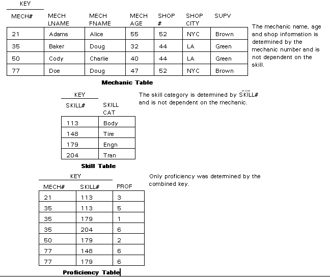 Figure C12 - Second Normal Form Relations
 Figure C12a - Mechanic Table
 Figure C12b - Skill Table
 Figure C12c - Proficiency Table
A relation is said to be in third normal form if it is in second normal form and there are no attributes (or sets of attributes) X and Y for which:
KEY X X Y
when X is not a candidate key.
Another way of looking at 3NF is that it results in relations that represent entities and relations that represent relationships among entities. An appropriate decomposition for converting a schema to third normal form is to place those attributes which are not directly (i.e., are only transitively) dependent on the key into a separate relation. The decompositions shown so far have two important features:
1.Each dependency is embodied in some relation (the decomposition preserves dependencies).
2.If an extension of the original relation is decomposed, it can be reconstructed via a JOIN of its components (the decomposition has lossless join).
In general, any relation schema can be decomposed into a third normal form schema that has lossless join and preserves dependencies.
 Figure C13 - Relations in Third Normal Form
The road to total normalization does not end here. Other anomalous situations may occur, and many other normal forms have been defined. Although six levels of normalization are possible, normalizing to 3NF is usually sufficient, and in some cases 2NF is sufficient.
What does normalization have to do with the design of database schemas? The answer is this: when designing schemas at the data level, the primary concern is not performance but, rather, integrity of the data involved. The study of normalization provides the designer of schemas at this level with a useful set of concepts which, by their very structure, support integrity and consistency of the data.